By going through these CBSE Class 12 Maths Notes Chapter 12 Linear Programming, students can recall all the concepts quickly.
Linear Programming Notes Class 12 Maths Chapter 12
Linear Programming Problems: Problems that minimize or maximize a linear function Z subject to certain conditions, determined by a set of linear inequalities with non-negative variables, are known as Linear Programming Problems.
Objective Function: A linear function Z = ax + by, where a and b are constants, which has to be maximized or minimized according to a set of given conditions, is called a linear objective function.
Decision Variables: In the objective function Z = ax + by, the variables x, y are said to be decision variables.
Constraints: The restrictions in the form of inequalities on the variables of linear programming problems are called constraints. The conditions x > 0, y > 0 are known as non-negative restrictions.
Example: A dealer deals in only two items: wall hangings and artificial plants. He has ₹ 5,000 to invest in and a space to store at the most 80 pieces. A wall hanging costs him ₹300 and an artificial plant ₹150. He can sell a wall hanging at a profit of ₹50 and an artificial plant at a profit of ₹18. Assuming he can sell all the items that he buys, formulate a linear programming problem in order to maximize his profit.
Let x be the number of wall hanging and y be the number of artificial plants.
Profit on one wall-hanging = ₹50.
∴ Profit by selling x wall hangings = ₹50x
Profit on one artificial plant = ₹18
∴ Profit by selling y artificial plants = ₹18y
The total profit = 50x + 18y
∴ Z = 50x + 18y is the objective function.
A wall hanging costs = ₹300.
∴ Cost of x wall-hangings = ₹300x
The cost of one artificial plant = ₹150
∴ Cost of y artificial plants = ₹150y
The total investment = ₹(300x + 150y)
But the maximum investment = ₹15000
⇒ 300x + 150y ≤ 15000
or
2x + y ≤ 100.
Further, storage capacity to a maximum is 80 pieces.
⇒ x + y ≤ 80.
We know that x ≥ 0, y ≥ 0
Thus, the constraints are 2x + y ≤ 100, x + y ≤ 80,
x ≥ 0, y ≥ 0
R Programming MCQ questions are useful for the campus placement for all freshers including experience professionals and engineers.
Graphical Method of solving a linear programming Problem:
In the above example, the constraints are 2x + y ≤ 100, x + y ≤ 80, x ≥ 0, y ≥ 0.
Now, we draw the lines 2x + y = 100, x + y = 80, x = 0, y = 0 and we find the regions which represent these inequalities.
(i) Consider the inequality
2x + y ≤ 100 .
The line 2x + y = 100 passes through A(50, 0) and B(0,100).
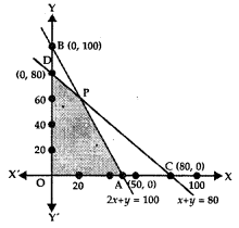
Putting x = 0, y = 0 in 2x + y ≤ 100, we get 0 ≤ 100, which is true.
This shows origin lies in this region, i.e., the region 2x + y ≤ 100 lies on and below AB as shown in the figure.
1. Next inequality is x + y ≤ 80.
The line x + y = 80 passes through C(80,0) and D(0, 80).
Putting x = 0, y = 0 in x + y < 80, we get 0 ≤ 80, which is true.
⇒ Origin lies in this region, i.e., the region x + y ≤ 80 is on and below CD.
(iii) x > 0 is the region on and to the right of the y-axis.
(iv) y > 0 is the region on and above the x-axis.
→ Feasible Region: The common region determined by all the constraints including non-negative constraints x, y > 0 of linear programming problem is known as feasible region.
In the figure drawn, the shaded area OAPD is the feasible region, which is the common area of the regions drawn under the given constraints.
→ Feasible Solution: Points within and on the boundary of the feasible region represents feasible solutions of constraints.
In the above figure, every point of the shaded area (feasible region) is the feasible solution.
In the feasible region, there are infinitely many points (solutions) that satisfy the given conditions. But we would like to know the points, where Z is maximum or minimum.
→ Theorem 1: Let R be the feasible region for a linear programming problem and let Z = ax + by be the objective function. When Z has an optimum value (maximum or minimum), where variables x and y are subject to constraints described by linear inequalities, the optimal value must occur at a corner point (vertex) of the feasible region.
→ Theorem 2: Let R be the feasible region for a linear programming problem and let Z = ax + by be the objective function. If R is bounded, then the objective function Z has both maximum and minimum value on R and each of these occurs at a corner point (vertex) of R.
Solving the equation 2x + y = 100 and x + y = 80, we get the coordinates of the point P(20, 60). •
In the example given above,
The values of Z at corner points are
At D (0, 80), Z = 50x + 18y = 18 × 80 – 1440
At P(20, 60), Z = 50 × 20 + 18 × 60 = 1000 + 1080 = 2080
At A(50, 0), Z = 50 × 50 + 0 = 2500
At 0(0, 0), Z = O.
Thus, the maximum value of Z is ₹2080 at P(20, 60) and the minimum value of Z is ₹1440 at D(0, 80). In fact, the minimum value is ₹0 at O.
However, if the feasible region is unbounded, the optimal value obtained may not be maximum or minimum.
To determine the optimal point, we proceed as follows:
- Let M be the maximum value found as explained above, if the open half-plane determined by ax + by > M has no point in common with the feasible region, then M is the maximum value of Z. Otherwise Z has no maximum value.
- Similarly, if m is the minimum value of Z and if the open half-plane determined by ax + by < m, has no point in common with the feasible region, then m is the minimum value of Z, otherwise, Z has no minimum value.
Different Types of Linear Programming Problems:
A few important linear programming problems are as follows:
1. Manufacturing Problem: In such a problem, we determine
- a number of units of different products to be produced and sold.
- Manpower required, Machine hours needed, warehouse space available, etc. The objective function is to maximize profit.
2. Diet Problem: Here we determine the number of different types of constituents or nutrients which should be included in the diet. The objective function is to minimize the cost of production.
3. Transportation Problems: These problems deal with the costs of transportation which are to be minimized under given constraints.
1. LINEAR PROGRAMMING
Linear programming is a too! which is used in decision making in business for obtaining maximum and minimum values of quantities subject to certain constraints.
2. MATHEMATICAL FORMULATION
Let the linear function Z be defined by :
(i) Z = c1 x1 + c2x2 + … + cnxn, where c’s are constants.
Let aij. be (mn) constants and bj. be a set of m constants such that:
a11x1 + a12 x2 + … + a1n xn (≤ , = ,≥) b1
a21x1 + a22 x2 + … + a2n xn (≤ , = ,≥) b2
………………………………..
………………………………..
am1x1 + am2 x2 + … + amn xn (≤ , = ,≥) bm
and let (iii) x1 ≥ 0, x1 ≥ 0, …, x ≥ 0.
The problem of determining the values of x , x^, …, x which maximizes (or minimizes) Z and satisfying above (ii) is called General Linear Programming Problem (LPP).
Note : In (ii), there may be any sign <. =, or >.
3. SOME DEFINITIONS
A. (i) Objective Function. The linear function Z = ax + by, where a, b are constants, which is to be maximized or minimized is called a linear objective function of LPP.
The variables x and y are called decision variables.
(ii) Constraints. The linear inequalities or inequations or restrictions on the variables of a linear programming problem are called constraints of LPP.
The conditions ,r > 0, y > 0 are called non-negative restrictions of LPP.
(iii) Optimization Problem. A problem, in which it is required to maximize or minimize a linear function (say of two variables x and y) subject to certain constraints, determined by a set of linear inequalities, is called the optimizations problem.
(iv) Solution. The values of x, y which satisfy the constraints of LPP is called the solution of the LPP.
(v) Feasible Solution. Any solution of LPP, which satisfies the non-negative restrictions of
the problem, is called a feasible solution to LPP.
(vi) Optimum Solution. Any feasible solution, which optimizes (minimizes or maximizes) the objective function of LPP is called an optimum solution of the general LPP.
B. (i) Feasible Region. The common region, which is determined by all the constraints including non-negative constraints x, y > 0 of a LPP is called feasible region (or solution region.) The region, other than the feasible one, is called an infeasible region.
(ii) Feasible Solution. The points, which lie on the boundary and within the feasible region, represent the feasible solution of the constraints.
Any part outside the feasible solution is called infeasible solution.
(iii) Optimal (Feasible) Solution. Any point in the feasible region, which gives the optimal value (maximum or minimum) of the objective function, is called optimal solution. These points are infinitely many in number.
Theorem I. Let R be the feasible region (convex polygon) for LPP and Z = ax + by, the objective function.
When Z has an optimal value (max. or min.) where x, y are subject to constraints, this optimal value will occur at a comer point (vertex).
Theorem II. Let R be the feasible region for LPP and Z = ax + by, the objecti ve function. If R is bounded , then the objective function Z has both maximum and minimum values of R and each occurs at a corner point (vertex).
Key Point
When R is unbounded, max. (or min.) value of objective function may not exist. In case it exists, it occurs at a comer point of R.
4. CORNER POINT METHOD
In order to solve a Linear Programming Problem we use Corner Point Method which is as below
Step I. Obtain the feasible region of LPP and determine its comer points (vertices).
Step II. Evaluate the objective function Z = ax + by at each comer point (vertex).
Let M and m be the largest and smallest values at these points.
Step III. (a) When the feasible region is bounded,
then M and m are the maximum and minimum values of Z.
(b) When the feasible region is unbounded, then
(i) M is the maximum value of Z if the open half-plane determined by ax + by > M has no common point with the feasible region; otherwise Z has no maximum value
(ii) m is the minimum value of Z if the open half-plane determined by ax + by < m has no common point with the feasible region; otherwise Z has no minimum value.