By going through these CBSE Class 12 Maths Notes Chapter 13 Probability, students can recall all the concepts quickly.
Probability Notes Class 12 Maths Chapter 13
1. Conditional Probability:
Let E and F be two events with a random experiment. Then, the probability of occurrence of E under the condition that F has already occurred and P(F) ≠ 0 is called the conditional probability. It is denoted by P(E/F).
The conditional probability P(E/F) is given by
P(E/F) = \(\frac{\mathrm{P}(\mathrm{E} \cap \mathrm{F})}{\mathrm{P}(\mathrm{F})}\) , when P(F) ≠ 0.
→ Properties:
- 0 ≤ P(E/F) ≤ 1
- P(F/F) = 1
- P(A ∪ B/F) = P(A/F) + P(B/F) – P(A n B/F)
If A and B are disjoint events,
then P(A ∪ B/F) = P(A/F) + P(B/F). - P(E/F) = 1 – P(E/F)
2. Multiplications Probability:
1. Multiplication Theorem on Probability:
Let E and F be two events associated with sample space S. P(E ∩ F) denotes the probability of the event that both E and F occur, which is given by P(E ∩ F) = P(E) P(F/E) = P(F) P(E/F) provided P(E) ≠ 0 and P(F) ≠ 0.
This result is known as the multiplication theorem on probability.
2. Multiplication rule of probability for more than two events:
Let E, F and G be the three events of sample space. Then, P(E ∩F ∩G) = P(E).P(F/E) P[G/(E ∩ F)]
3. Independent Events:
- Two events E and F are said to be independent, if P(E/F) = P(E) and P(F/E) = P(F), provided P(E) ≠ 0 and P(F) ≠ 0.
We know that P(E ∩ F)= P(E). P(F/E) and P(E ∩ F) = P(F). P(E/F). - Events E and F are independent if P(E ∩ F) = P(E) × P(F).
- Three events E, F and G are said to be independent or mutually independent, if
P(E∩F∩G)= P(E). P(F). P(G)
4. Partition of a Sample Space:
A set of events E1, E2,……….., En is said to represent a partition of sample S, if
- Ei ∩ Fj = Φ, if i ≠ j, i, j = 1, 2,……….. ,n .
- E1 ∪ E2 ∪ E3 ∪ …. ∪ En = S
- P(Ei) > 0 for all i = 1, 2,……., n
For example, E and E’ (complement of E) form a partition of sample space S, because
E∩E’ = Φ and E∪E’ = S.
5. Theorem of Total Probability:
Let E1, E2,…….., En be a partition of sample space and each event has a non-zero probability.
If A be any event associated with S, then
P(A) = P(E1) P(A/E1) + P(E2) P(A/E2) + P(E3) P(A/E3) +…….. + P(En) P(A/En)
![]()
6. Bayes’ Theorem:
Let E1, E2,…………, En be the n events forming a partition of sample space S, i.e., E1, E2,………, E( are pairwise disjoint and E1 ∪ E2 ∪………. ∪
En = S and A is any event of non-zero probability, then

7. A Few Terminologies:
- Hypothesis: When Bayes’ Theorem is applied, the events E1, E2,……………., En is said to be a hypothesis.
- Priori Probability: The probabilities P(E1), P(E2),…………., P(En) is called priori.
- Posteriori Probability: The conditional probability P(E./A) is known as the posterior probability of hypothesis E.
8. Random Variable:
A random variable is a real-valued function whose domain is the sample space of a random experiment.
For example, let us consider the experiment of tossing a coin three times.
The sample space of the experiment is
S{TTT, TTH, THT, HTT, HHT, HTH, THH, HHH}
If x denotes the number of heads obtained, then X is the random variable for each outcome.
X(0) = {TTT}
X(1) = {TTH, THT, HTT}
X(2) = {HHT, HTH, THH}
X(3) = {HHH}
9. Probability Distribution of a Random Variable:
Let real numbers x1, x2,…………., xn be the possible values of random variable and p1, p2,……………, pn be probabilities corresponding to each value of the random variable X. Then the probability distribution is

It may be noted that
- pi > 0
- Sum of probabilities p1 + p2 +………….+ pn = 1
Example: Three cards are drawn successively with replacement from a well-shuffled pack of 52 cards. A random variable denotes the number of spades on three cards. Determine the probability distribution of X.
P(S) = P(Drawing a spade) = \(\frac{13}{52}=\frac{1}{4}\)
P(F) = P(Drawing not a space = 1 – \(\frac{1}{4}=\frac{3}{4}\)
P(X = 0) =P(FFF) = \(\left(\frac{3}{4}\right)^{3}=\frac{27}{64}\)
P(X = 1) = 3 × \(\left(\frac{1}{4} \times \frac{3}{4} \times \frac{3}{4}\right)=\frac{27}{64}\)
∵ X = 1 ⇒{SFF, FSF, FFS}
X = 2 ⇒ {SSF, SFS, FSS}
∴ P(X – 2) = 3 × \(\left(\frac{1}{4} \times \frac{1}{4} \times \frac{3}{4}\right)=\frac{9}{64}\)
When X = 3 ⇒ {SSS}
P(X = 3) = \(\frac{1}{4} \times \frac{1}{4} \times \frac{1}{4}=\frac{1}{64}\)
∴ Probability distribution is

10. Mean of Random Variable:
Let X be the random variable whose possible values are x1, x2,……….,xn. If p1, p2,……….., pn are the corresponding probabilities, then the mean of X denoted by p is given by
![]() |
|
The mean of a random variable X is also called the expected value of X, denoted by E(x).
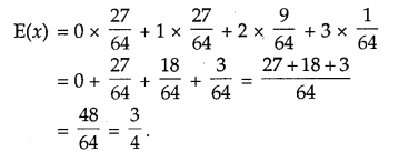
For the experiment of drawing a spade in three cards, the expected value ‘

11. Variance of a Random Variable:
Let X be the random variable with possible values of X: x1 x2,……xn occur whose probabilities are p1, p2,………., pn respectively.
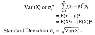
Let μ = E(x) be the mean of X. The variance of X, denoted by Var (X) or σx2, is defined as

12. Bernoulli Trial:
Trials of a random experiment are said to be Bernoulli’s Trials if they satisfy the following conditions:
- The trials should be independent.
- Each trial has exactly two outcomes viz. success or failure.
- The probability of success remains the same in each trial.
- The number of trials is finite.
Example: An urn contains 6 red and 5 white balls. Four balls are drawn successively. Find whether the trials of drawing balls are Bernoulli trials when after each draw the ball draw is
- replaced
- not replaced in the urn.
1. If drawing a red ball with replacement is a success, in each trial the probability of success = \(\frac{6}{11}\).
Therefore, drawing a ball with replacement is a Bernoulli trial.
2. In the second attempt, when the ball is not replaced, the probability of success = \(\frac{5}{10}\).
In thired attempt, the probability of success = \(\frac{4}{9}\).
Thus, probability changes at each trial. Hence, in this case, it is not a Bernoulli trial.
13. Binomial Distribution:
The probability distribution of a number of successes in an experiment consisting of n Bernoulli trials is obtained by binomial expansion of (q + p)n.
Such a probability distribution may be written as:

This probability distribution is called binomial distribution with parameters n and p.
14. Probability Function:
The probability of x success is denoted by P(x). In a binomial distribution P(x) is given by
P(x) = nCx qn-x px, x = 0,1, 2,…., n and q = 1 – p.
The function P(x) is known as the probability function of the binomial distribution.
1. DEFINITIONS
(i) Random Experiment of Trial. The performance of an experiment is called a trial.
(ii) Event. The possible outcomes of a trial are called events.
(iii) Equally likely Events. The events are said to be equally likely if there is no reason to expect
any one in preference to any other.
(iv ) Exhaustive Events. It is the total number of all possible outcomes of any trial.
(v) Mutually Exclusive Events. Two or more events are said to be mutually exclusive if they
cannot happen simultaneously in a trial. s:
(vi) Favourable Events. The cases which ensure the occurrence of the events are called favourable.
(vii) Sample Space. The set of all possible outcomes of an experiment is called a sample space.
( viii) Probability of occurrences of event A, denoted by P (A), is defined as :
P(A) = \(\frac{\text { No. of favourable cases }}{\text { No. of exhaustive cases }}=\frac{n(\mathrm{~A})}{n(\mathrm{~S})}\)
2. THEOREMS .
(i) In a random experiment, if S be the sample space and A an event, then :
(I) P (A) ≥ 0. (II) P (Φ) = 0 and (III) P (S) = 1.
(ii) If A and B are mutually exclusive events, then P (A ∩ B) = 0.
(iii) If A and B are two mutually exclusive events, then P (A) + P (B) – 1.
(iv) If A and B are mutually exclusive events, then : P (A ∪ B) = P ( A) + P ( B). s
(v) For any two events A and B. P (A ∪ B) = P (A) + P (B) – P (A ∩ B).
(vi) For each event A. P (\(\overline{\mathrm{A}}\)) = 1 – P (A), where (\(\overline{\mathrm{A}}\)) is the complementary event. 1;
( vii) 0 ≤ P (A) ≤ 1.
3. MORE DEFINITIONS
(i) Compound Event. The simultaneous happening of two or more events is called a compound event if they occur in connection with each other. I
(ii) Conditional Probability. Let A and B be two events associated with the same sample spat e then
P (A/B) = \(\frac { No. of elementary events favourable to B which are also favourable to A }{ No. of elementary events favourable to B }\)
Theorem. P (A/B) = \(\frac{P(A \cap B)}{P(B)}\)
P(B/A) = \(\frac{P(A \cap B)}{P(A)}\)
(iii) Independent Events. Two events are said to be independent if the occurrence of one does not a depend upon the occurrence of the other.
Theorem. P (A ∩ B) = P (A) P (B) when A, B are independent.
4. If A1, A1, …………Ar be r events, then the probability when at least one event happens
= 1 – \(\mathbf{P}\left(\overline{\mathbf{A}_{1}}\right) \mathrm{P}\left(\overline{\mathbf{A}_{2}}\right) \ldots \cdot \mathbf{P}\left(\overline{\mathrm{A}}_{r}\right)\)
5. BAYES’ FORMULA
If E1, E2,…., En are mutually exclusive and exhaustive events and A is any event that occurs with E1, E2, …. , En, then :
P(E1/A) = \(\frac{\mathrm{P}\left(\mathrm{E}_{1}\right) \mathrm{P}\left(\mathrm{A} / \mathrm{E}_{1}\right)}{\mathrm{P}\left(\mathrm{E}_{1}\right) \mathrm{P}\left(\mathrm{A} / \mathrm{E}_{1}\right)+\mathrm{P}\left(\mathrm{E}_{2}\right) \mathrm{P}\left(\mathrm{A} / \mathrm{E}_{2}\right)+\ldots \ldots \ldots+\mathrm{P}\left(\mathrm{E}_{n}\right) \mathrm{P}\left(\mathrm{A} / \mathrm{E}_{n}\right)}\)
6. MEAN AND VARIANCE OF RANDOM VARIABLE.
Mean (μ) = Σxipi
Variance (σ2) = Σ(xi – μ)2pi = Σxi2 pi – μ2