Prasanna

Find free online Chemistry Topics covering a broad range of concepts from research institutes around the world.

Periodic Trends in Chemical Properties:

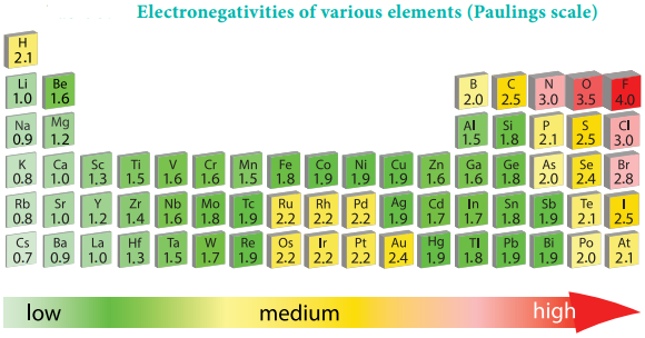
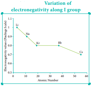
So far, we have studied the periodicity of the physical properties such as atomic radius, ionisation enthalpy, electron gain enthalpy and electronegativity. In addition, the chemical properties such as reactivity, valence, oxidation state etc… also show periodicity to certain extent.

In this section, we will discuss briefly about the periodicity in valence (oxidation state) and anomalous behaviour of second period elements (diagonal relationship).

Valence or Oxidation States

The valence of an atom is the combining capacity relative to hydrogen atom. It is usually equal to the total number of electrons in the valence shell or equal to eight minus the number of valence electrons. It is more convenient to use oxidation state in the place of valence.

Periodicity of Valence or Oxidation States

The valence of an atom primarily depends on the number of electrons in the valence shell. As the number of valence electrons remains same for the elements in same group, the maximum valence also remains the same. However, in a period the number of valence electrons increases, hence the valence also increases.

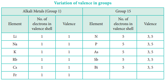
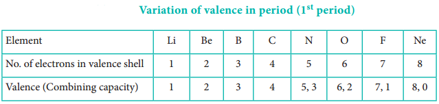
In addition to that some elements have variable valence. For example, most of the elements of group 15 which have 5 valence electrons show two valences 3 and 5. Similarly transition metals and inner transition metals also show variable oxidation states.

Anomalous Properties of Second Period Elements:

As we know, the elements of the same group show similar physical and chemical properties. However, the first element of each group differs from other members of the group in certain properties. For example, lithium and beryllium form more covalent compounds, unlike the alkali and alkali earth metals which predominantly form ionic compounds.

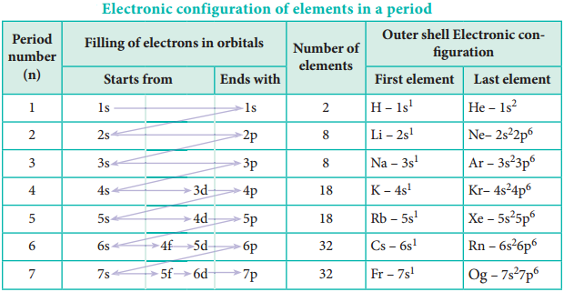
The elements of the second period have only four orbitals (2s & 2p) in the valence shell and have a maximum co-valence of 4, whereas the other members of the subsequent periods have more orbitals in their valence shell and shows higher valences. For example, boron forms BF₄^– and aluminium forms AlF₆^3-.

Diagonal Relationship

On moving diagonally across the periodic table, the second and third period elements show certain similarities. Even though the similarity is not same as we see in a group, it is quite pronounced in the following pair of elements.

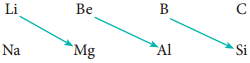
The similarity in properties existing between the diagonally placed elements is called ‘diagonal relationship’.

Periodic Trends and Chemical Reactivity:

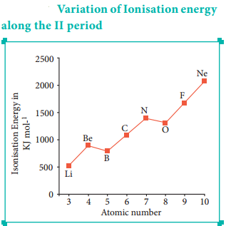
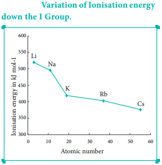
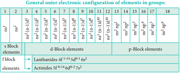
The physical and chemical properties of elements depend on the valence shell electronic configuration as discussed earlier. The elements on the left side of the periodic table have less ionisation energy and readily lose their valence electrons.

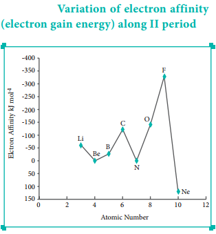
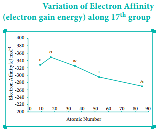
On the other hand, the elements on right side of the periodic table have high electron affinity and readily accept electrons. As a consequence of this, elements of these extreme ends show high reactivity when compared to the elements present in the middle. The noble gases having completely filled electronic configuration neither accept nor lose their electron readily and hence they are chemically inert in nature.

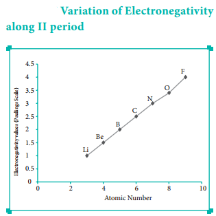
The ionisation energy is directly related to the metallic character and the elements located in the lower left portion of the periodic table have less ionisation energy and therefore show metallic character. On the other hand the elements located in the top right portion have very high ionisation energy and are nonmetallic in nature.

Let us analyse the nature of the compounds formed by elements from both sides of the periodic table. Consider the reaction of alkali metals and halogens with oxygen to give the corresponding oxides.

4 Na + O₂ → 2 Na₂O
2 Cl₂ + 7O₂ → 2 Cl₂O₇

Since sodium oxide reacts with water to give strong base sodium hydroxide, it is a basic oxide. Conversely Cl₂O₇ gives strong acid called perchloric acid upon reaction with water So, it is an acidic oxide.

Na₂O + H₂O → 2NaOH
Cl₂O₇ → 2 Cl₂O₇

Thus, the elements from the two extreme ends of the periodic table behave differently as expected. As we move down the group, the ionisation energy decreases and the electropositive character of elements increases. Hence, the hydroxides of these elements become more basic. For example, let us consider the nature of the second group hydroxides:

Be(OH)₂ amphoteric; Mg(OH)₂ weakly basic; Ba(OH)₂ strongly basic

Beryllium hydroxide reacts with both acid and base as it is amphoteric in nature.

Be(OH)₂ + 2HCl → BeCl₂ + 2H₂O
Be(OH)₂+ 2 NaOH → Na₂BeO₂ + 2H₂O.

Find free online Chemistry Topics covering a broad range of concepts from research institutes around the world.

Periodic Trends in Properties

As discussed earlier, the electronic configuration of the elements shows a periodic variation with increase in atomic numbers. Similarly a periodic trend is observed in physical and chemical behaviour of elements. In this section, we will study the periodic trends in the following properties of elements.

• Atomic Radius
• Ionic Radius
• Ionisation Enthalpy (energy)
• Electron Gain Enthalpy (Electron Affinity)
• Electronegativity

Atomic Radius

Atomic radius of an atom is defined as the distance between the centre of its nucleus and the outermost shell containing the valence electron.

It is not possible to measure the radius of an isolated atom directly. Except for noble gases, usually atomic radius is referred to as covalent radius or metallic radius depending upon the nature of bonding between the concerned atoms.

Covalent Radius

It is one-half of the internuclear distance between two identical atoms linked together by a single covalent bond. Inter nuclear distance can be determined using x-ray diffraction studies.

Example:

The experimental internuclear distance in Cl₂ molecule is 1.98 Å. The covalent radius of chlorine is calculated as below.

d_Cl-Cl = r_Cl + r_Cl
⇒ d_Cl-Cl = 2r_Cl

The formation of covalent bond involves the overlapping of atomic orbitals and it reduces the expected internuclear distance. Therefore covalent radius is always shorter than the actual atomic radius.

In case of hetero nuclear diatomic molecules, the covalent radius of individual atom can also be calculated using the internuclear distance (d_A-B) between two different atoms A and B. The simplest method proposed by Schomaker and Stevenson is as follows.

d_A-B = r_A + r_B – 0.09 (x_A – x_B)

where χ_A and χ_B are the electronegativities of A and B respectively in Pauling units. Here χ_A > χ_B and
radius is in Å.

Let us calculate the covalent radius of hydrogen using the experimental d_H-Cl value is 1.28 Å and the covalent radius of chlorine is 0.99 Å. In pauling scale the electronegativity of chlorine and hydrogen are 3 and 2.1 respectively.

d_H-Cl = r_H + r_Cl – 0.09 (x_Cl – x_H)
1.28 = r_H + 0.99 – 0.09 (3 – 2.1)
1.28 = r_H + 0.99 – 0.09 (0.9)
1.28 = r_H + 0.99 – 0.081
1.28 = r_H + 0.909
∴ r_H = 1.28 – 0.909 = 0.371 Å

Metallic Radius

It is defied as one-half of the distance between two adjacent metal atoms in the closely packed metallic crystal lattice. For example, the distance between the adjacent copper atoms in solid copper is 2.56 Å and therefore the metallic radius of copper is \(\frac{2.56}{2}\) = 1.28 Å

The metallic radius can be calculated using the unit cell length of the metallic crystal. You will study the detailed calculation procedure in XII standard solid state unit.

Periodic Trends in Atomic Radius

Variation in Periods

Atomic radius tends to decrease in a period. As we move from left to right along a period, the valence electrons are added to the same shell. The simultaneous addition of protons to the nucleus, increases the nuclear charge, as well as the electrostatic attractive force between the valence electrons and the nucleus. Therefore atomic radius decreases along a period.

Effective Nuclear Charge

In addition to the electrostatic forces of attraction between the nucleus and the electrons, there exists repulsive forces among the electrons. The repulsive force between the inner shell electrons and the valence electrons leads to a decrease in the electrostatic attractive forces acting on the valence electrons by the nucleus. Thus, the inner shell electrons act as a shield between the nucleus and the valence electrons. This effect is called shielding effect.

The net nuclear charge experienced by valence electrons in the outermost shell is called the effective nuclear charge. It is approximated by the below mentioned equation.

Z_eff = Z – S

Where Z is the atomic number and ‘S’ is the screening constant which can be calculated using Slater’s rules as described below.

Step 1:

Write the electronic configuration of the atom and rearrange it by grouping ns and np orbitals together and others separately in the following form. (1s) (2s, 2p) (3s, 3p) (3d) (4s, 4p) (4d) (4f) (5s, 5p) …

Step 2:

Identify the group in which the electron of interest is present. The electron present right to this group does not contribute to the shielding effect. Each of the electrons within the identified group (denoted by ‘n’) shields to an extent of 0.35 unit of nuclear charge. However, it is 0.30 unit for 1s electron.

Step 3:

Shielding of inner shell electrons. If the electron of interest belongs to either s or p orbital,

• Each electron within the (n-1) group shields to an extent of 0.85 unit of nuclear charge, and
• Each electron within the (n-2) group (or) even lesser group (n-3), (n-4) etc … completely shields i.e. to an extent of 1.00 unit of nuclear charge.

If the electron of interest belongs to d or f orbital, then each of electron left of the group of electron of interest shields to an extent of 1.00 unit of nuclear charge.

Step 4:

Summation of the shielding effect of all the electrons gives the shielding constant ‘S’

Example:

Let us explain the calculation of effective nuclear charge on 4s electron and 3d electron in scandium. The electronic configuration of scandium is 1s², 2s², 2p⁶, 3s², 3p⁶, 4s², 3d¹. we can rearrange as below.

Calculation of Effective Nuclear Charge on 3d Electron

∴ Z_eff = Z – S i.e. = 21 – 8 ∴Z_eff = 3

Variation in Group

In the periodic table, the atomic radius of elements increases down the group. As we move down a group, new shells are opened to accommodate the newly added valence electrons. As a result, the distance between the centre of the nucleus and the outermost shell containing the valence electron increases. Hence, the atomic radius increases. The trend in the variation of the atomic radius of the alkali metals down the group os shown below.

Ionic Radius

It is defined as the distance from the centre of the nucleus of the ion up to which it exerts its influence on the electron cloud of the ion. Ionic radius of uni-univalent crystal can be calculated using Pauling’s method from the inter ionic distance between the nuclei of the cation and anion. Pauling assumed that ions present in a crystal lattice are perfect spheres, and they are in contact with each other. Therefore,

d = r_C⁺ + r_A^– ………………… (1)

Where d is the distance between the centre of the nucleus of cation C⁺ and anion A^– and r_C⁺, r_A^– are the radius of the cation and anion respectively.

Pauling also assumed that the radius of the ion having noble gas electronic configuration (Na⁺ and Cl^– having
1s² 2s², 2p⁶ configuration) is inversely proportional to the effective nuclear charge felt at the periphery of
the ion.

Where Z_eff is the effective nuclear charge and Z_eff = Z – S

Dividing the equation 2 by 3

On solving equation (1) and (4) the values of r_C⁺ and r_A^– can be obtained

Let us explain this method by calculating the ionic radii of Na⁺ and F^– in NaF crystal whose interionic distance is equal to 231 pm.

Ionisation Energy

It is defined as the minimum amount of energy required to remove the most loosely bound electron from the valence shell of the isolated neutral gaseous atom in its ground state. It is expressed in kJ mol^-1 or in electron volts (eV). M_(g) + IE₁ → M⁺_(g) + 1 e^–

Successive Ionisation Energies

The minimum amount of energy required to remove an electron from a unipositive cation is called second ionisation energy. It is represented by the following equation.

M⁺_(g) + IE₂ → M²⁺_(g) + 1e^–

In this way we can define the successive ionisation energies such as third, fourth etc.

The total number of electrons are less in the cation than the neutral atom while the nuclear charge remains the same. Therefore the effective nuclear charge of the cation is higher than the corresponding neutral atom. Thus the successive ionisation energies, always increase in the following order

IE₁ < IE₂ < IE₃ < …..

Periodic Trends in Ionisation Energy

The ionisation energy usually increases along a period with few exceptions. As discussed earlier, when we move from left to right along a period, the valence electrons are added to the same shell, at the same time protons are added to the nucleus.

This successive increase of nuclear charge increases the electrostatic attractive force on the valence electron and more energy is required to remove the valence electron resulting in high ionisation energy.

Let us consider the variation in ionisation energy of second period elements. The plot of atomic number vs ionisation energy is given below.

In the following graph, there are two deviation in the trends of ionisiation energy. It is expected that boron has higher ionisation energy than beryllium since it has higher nuclear charge. However, the actual ionisation energies of beryllium and boron are 899 and 800 kJ mol^-1 respectively contrary to the expectation. It is due to the fact that beryllium with completely filled 2s orbital, is more stable than partially filled valence shell electronic configuration of boron. (2s², 2p¹)

The electronic configuration of beryllium (Z=4) in its ground state is 1s², 2s² and that of boran is (Z = 5) 1s² 2s² 2p¹

Similarly, nitrogen with 1s², 2s², 2p³ electronic configuration has higher ionisation energy (1402 kJ mol^-1) than oxygen (1314 kJ mol^-1). Since the half filled electronic configuration is more stable, it requires higher energy to remove an electron from 2p orbital of nitrogen. Whereas the removal one 2p electron from oxygen leads to a stable half filled configuration. This makes comparatively easier to remove 2p electron from oxygen.

Periodic Variation in Group

The ionisation energy decreases down a group. As we move down a group, the valence electron occupies new shells, the distance between the nucleus and the valence electron increases. So, the nuclear forces of attraction on valence electron decreases and hence ionisation energy also decreases down a group.

Ionisation Energy and Shielding Effect

As we move down a group, the number of inner shell electron increases which in turn increases the repulsive force exerted by them on the valence electrons, i.e. the increased shielding effect caused by the inner electrons decreases the attractive force acting on the valence electron by the nucleus. Therefore the ionisation energy decreases. Let us understand this trend by considering the ionisation energy of alkali metals.

Electron Affinity

It is defined as the amount of energy released (required in the case noble gases) when an electron is added to the valence shell of an isolated neutral gaseous atom in its ground state to form its anion. It is expressed in kJ mol^-1

A + e^– → A^– + EA

Variation of Electron Affinity in a Period:

The variation of electron affinity is not as systematic as in the case of ionisation energy. As we move from alkali metals to halogens in a period, generally electron affinity increases, i.e. the amount of energy released will be more. This is due to an increase in the nuclear charge and decrease in size of the atoms.

However, in case of elements such as beryllium (1s², 2s²), nitrogen (1s², 2s², 2p³) the addition of extra electron will disturb their stable electronic configuration and they have almost zero electron affinity.

Noble gases have stable ns², np⁶ configuration, and the addition of further electron is unfavourable and requires energy. Halogens having the general electronic configuration of ns², np⁵ readily accept an electron to get the stable noble gas electronic configuration (ns², np⁶), and therefore in each period the halogen has high electron affinity. (high negative values)

Variation of Electron Affinity in a Group:

As we move down a group, generally the electron affinity decreases. It is due to increase in atomic size and the shielding effect of inner shell electrons. However, oxygen and fluorine have lower affinity than sulphur and chlorine respectively.

The sizes of oxygen and fluorine atoms are comparatively small and they have high electron density. Moreover, the extra electron added to oxygen and fluorine has to be accommodated in the 2p orbital which is relatively compact compared to the 3p orbital of sulphur and chlorine so, oxygen and fluorine have lower electron affinity than their respective group elements sulphur and chlorine.

Electronegativity

It is defined as the relative tendency of an element present in a covalently bonded molecule, to attract the shared pair of electrons towards itself. Electronegativity is not a measurable quantity. However, a number of scales are available to calculate its value. One such method was developed by Pauling, he assigned arbitrary value of electronegativities for hydrogen and fluorine as 2.1 and 4.0 respectively. Based on this the  electronegativity values for other elements can be calculated using the following expression

Where E_AB, E_AA and E_BB are the bond dissociation energies (K cal) of AB, A₂ and B₂ molecules respectively.

The electronegativity of any given element is not a constant and its value depends on the element to which it is covalently bound. The electronegativity values play an important role in predicting the nature of the bond.

Variation of Electronegativity in a Period:

The electronegativity generally increases across a period from left to right. As discussed earlier, the atomic radius decreases in a period, as the attraction between the valence electron and the nucleus increases. Hence the tendency to attract shared pair of electrons increases. Therefore, electronegativity also increases in a period.

Variation of Electronegativity in a Group:

The electronegativity generally decreases down a group. As we move down a group the atomic radius increases and the nuclear attractive force on the valence electron decreases. Hence, the electronegativity decreases.

Noble gases are assigned zero electronegativity. The electronegativity values of the elements of s-block show the expected decreasing order in a group. Except 13^th and 14^th group all other p-block elements follow the expected decreasing trend in electronegativity.

Find free online Chemistry Topics covering a broad range of concepts from research institutes around the world.

Grouping of Elements Based on Electronic Configurations

In the modern periodic table, the elements are organised in 7 periods and 18 groups based on the modern periodic law. The placement of element in the periodic table is closely related to its outer shell electronic configuration. Let us analyse the change in the electronic configuration of elements along the periods and down the groups.

Variation of Electronic Configuration Along the Periods

We have already learnt that each period starts with the element having general outer electronic configuration ns¹ and ends with ns², np⁶ where n is the period number. The first period starts with the filling of valence electrons in 1s orbital, which can accommodate only two electrons.

Hence, the first period has two elements, namely hydrogen and helium. The second period starts with the filling of valence electrons in 2s orbital followed by three 2p orbitals with eight elements from lithium to neon. The third period starts with filling of valence electrons in the 3s orbital followed by 3p orbitals.

The fourth period starts with filling of valence electrons from 4s orbital followed by 3d and 4p orbitals in accordance with Aufbau principle. Similarly, we can explain the electronic configuration of elements in the subsequent periods (Table 3.10).

In the fourth period the filling of 3d orbitals starts with scandium and ends with zinc. These 10 elements are called first transition series. Similarly 4d, 5d and 6d orbitals are filled in successive periods and the corresponding series of elements are called second, third and fourth transition series respectively.

In the sixth period the filling of valence electrons starts with 6s orbital followed by 4f, 5d and 6p orbitals. The filling up of 4f orbitals begins with Cerium (Z=58) and ends at Lutetium (Z=71). These 14 elements constitute the first inner-transition series called Lanthanides.

Similarly, in the seventh period 5f orbitals are filled, and it’s -14 elements constitute the second inner transition series called Actinides. These two series are placed separately at the bottom of the modern periodic table.

Variation of Electronic Configuration in the Groups:

Elements of a group have similar electronic configuration in the outer shell. The general outer electronic configurations for the 18 groups are listed in the Table 3.11. The groups can be combined as s, p, d and f block elements on the basis of the orbital in which the last valence electron enters.

The elements of group 1 and group 2 are called s-block elements, since the last valence electron enters the ns orbital. The group 1 elements are called alkali metals while the group 2 elements are called alkaline earth metals.

These are soft metals and possess low melting and boiling points with low ionisation enthalpies. They are highly reactive and form ionic compounds. They are highly electropositive in nature and most of the elements imparts colour to the flame. We will study the properties of these group elements in detail in subsequent chapters.

The elements of groups 13 to 18 are called p-block elements or representative elements and have a general electronic configuration ns², np^1-6. The elements of the group 16 and 17 are called chalcogens and halogens respectively.

The elements of 18^th group contain completely filled valence shell electronic configuration (ns², np⁶) and are called inert gases or nobles gases. The elements of p-block have high negative electron gain enthalpies. The ionisation energies are higher than that of s-block elements. They form mostly covalent compounds and shows more than one oxidation states in their compounds.

The elements of the groups 3 to 12 are called d-block elements or transition elements with general valence shell electronic configuration ns^1-2, (n-1)d^1-10. These elements also show more than one oxidation state and form ionic, covalent and co-ordination compounds. They can form interstitial compounds and alloys which can also act as catalysts. These elements have high melting points and are good conductors of heat and electricity.

The lanthanides (4f^1-14, 5d^0-1, 6s²) and the actinides (5f^0-14, 6d^0-2, 7s²) are called f-block elements. These elements are metallic in nature and have high melting points. Their compounds are mostly coloured. These elements also show variable oxidation states.

Find free online Chemistry Topics covering a broad range of concepts from research institutes around the world.

Nomenclature of Elements with Atomic Number Greater than 100

Usually, when a new element is discovered, the discoverer suggests a name following IUPAC guidelines which will be approved after a public opinion. In the meantime, the new element will be called by a temporary name coined using the following IUPAC rules, until the IUPAC recognises the new name.

1. The name was derived directly from the atomic number of the new element using the following numerical roots.

Notation for IUPAC Nomenclature of Elements

2. The numerical roots corresponding to the atomic number are put together and ‘ium’ is added as suffix

3. The final ‘n’ of ‘enn’ is omitted when it is written before ‘nil’ (enn + nil = enil) similarly the final ‘i’ of ‘bi’ and ‘tri’ is omitted when it written before ‘ium’ (bi + ium = bium; tri + ium = trium)

4. The symbol of the new element is derived from the first letter of the numerical roots.

The following table illustrates these facts.

To overcome all these difficulties, IUPAC nomenclature has been recommended for all the elements with Z > 100. It was decided by IUPAC that the names of elements beyond atomic number 100 should use Latin words for their numbers. The names of these elements are derived from their numerical roots.

Fermium is a synthetic element with the symbol Fm and atomic number 100. It is an actinide and the heaviest element that can be formed by neutron bombardment of lighter elements, and hence the last element that can be prepared in macroscopic quantities, although pure fermium metal has not yet been prepared.

The twelve elements of nature are Earth, Water, Wind, Fire, Thunder, Ice, Force, Time, Flower, Shadow, Light and Moon.

Uranium

The heaviest element known to occur in nature is uranium, which contains only 92 protons, putting it 30 places below the putative new element in the periodic table. In the laboratory, physicists have managed to create elements up to 118, but they are all highly unstable.

The fifth element on top of earth, air, fire, and water, is space or aether. It was hard for people to believe that the stars and everything else in space were made of the other elements, so space was considered as a fifth element.

According to ancient and medieval science, aether also spelled ether, aither, or ether and also called quintessence (fifth element), is the material that fills the region of the universe above the terrestrial sphere.

Find free online Chemistry Topics covering a broad range of concepts from research institutes around the world.

Moseley’s Work and Modern Periodic Law

In 1913, Henry Moseley studied the characteristic X-rays spectra of several elements by bombarding them with high energy electrons and observed a linear correlation between atomic number and the frequency of X-rays emitted which is given by the following expression.

\(\sqrt{υ}\) = a(Z – b)

Where, υ is the frequency of the X-rays emitted by the element with atomic number ‘Z’; a and b are constants and have same values for all the elements.

The plot of \(\sqrt{υ}\) against Z gives a straight line. Using this relationship, we can determine the atomic number of an unknown (new) element from the frequency of X-ray emitted. Based on his work, the modern periodic law was developed which states that, “the physical and chemical properties of the elements are periodic functions of their atomic numbers.” Based on this law, the elements were arranged in order of their increasing atomic numbers.

This mode of arrangement reveals an important truth that the elements with similar properties recur after regular intervals. The repetition of physical and chemical properties at regular intervals is called periodicity.

Modern Periodic Table

The physical and chemical properties of the elements are correlated to the arrangement of electrons in their outermost shell (valence shell). Different elements having similar outer shell electronic configuration possess similar properties. For example, elements having one electron in their valence shell s-orbital possess similar physical and chemical properties. These elements are grouped together in the modern periodic table as first group elements.

Similarly, all the elements are arranged in the modern periodic table which contains 18 vertical columns and 7 horizontal rows. The vertical columns are called groups and the horizontal rows are called periods. Groups are numbered 1 to 18 in accordance with the IUPAC recommendation which replaces the old numbering scheme IA to VIIA, IB to VIIB and VIII.

Each period starts with the element having general outer electronic configuration ns¹ and ends with ns² np⁶.
Here ‘n’ corresponds to the period number (principal quantum number). The aufbau principle and the  electronic configuration of atoms provide a theoretical foundation for the modern periodic table.

Find free online Chemistry Topics covering a broad range of concepts from research institutes around the world.

Classification of Elements

During the 19^th century, scientists have isolated several elements and the list of known elements increased. Currently, we have 118 known elements. Out of 118 elements, 92 elements with atomic numbers 1 to 92 are found in nature. Scientists have found out there are some similarities in properties among certain elements.

This observation has led to the idea of classification of elements based on their properties. In fact, classification will be beneficial for the effective utilization of these elements. Several attempts were made to classify the elements. However, classification based on the atomic weights led to the construction of a proper form of periodic table.

In 1817, J. W. Dobereiner classified some elements such as chlorine, bromine and iodine with similar chemical properties into the group of three elements called as triads. In triads, the atomic weight of the middle element nearly equal to the arithmetic mean of the atomic weights of the remaining two elements. However, only a limited number of elements can be grouped as triads.

This concept can not be extended to some triads which have nearly same atomic masses such as [Fe, Co, Ni], [Ru, Rh, Pd] and [Os, Ir, Pt].

In 1862, A. E. B. de Chancourtois reported a correlation between the properties of the elements and their atomic weights. He said ‘the properties of bodies are the properties of numbers’. He intended the term numbers to mean the value of atomic weights.

He designed a helix by tracing at an angle 45˚ to the vertical axis of a cylinder with circumference of 16 units. He arranged the elements in the increasing atomic weights along the helix on the surface of this cylinder.

One complete turn of a helix corresponds to an atomic weight increase of 16. Elements which lie on the 16 equidistant vertical lines drawn on the surface of cylinder shows similar properties. This was the first reasonable attempt towards the creation of periodic table. However, it did not attract much attention.

In 1864, J. Newland made an attempt to classify the elements and proposed the law of octaves. On arranging the elements in the increasing order of atomic weights, he observed that the properties of every eighth element are similar to the properties of the first element. This law holds good for lighter elements up to calcium.

Mendeleev’s Classification

In 1868, Lothar Meyer had developed a table of the elements that closely resembles the modern periodic table. He plotted the physical properties such as atomic volume, melting point and boiling point against atomic weight and observed a periodical pattern.

During same period Dmitri Mendeleev independently proposed that “the properties of the elements are the periodic functions of their atomic weights” and this is called periodic law. Mendeleev listed 70 elements, which were known till histime in several vertical columns in order of increasing atomic weights. Thus, Mendeleev constructed the first periodic table based on the periodic law.

As shown in the periodic table, he left some blank spaces since there were no known elements with the appropriate properties at that time. He and others predicted the physical and chemical properties of the missing elements. Eventually these missing elements were discovered and found to have the predicted properties.

For example, Gallium (Ga) of group III and germanium (Ge) of group IV were unknown at that time. But Mendeleev predicted their existence and properties. He referred the predicted elements as eka-aluminium and eka-silicon. After discovery of the actual elements, their properties were found to match closely to those predicted by Mendeleev (Table 3.4).

Properties predicted for Eka-aluminium and Eka-silicon

Anomalies of Mendeleev’s Periodic Table

Some elements with similar properties were placed in different groups and those with dissimilar properties were placed in same group. Similarly elements with higher atomic weights were placed before lower atomic weights based on their properties in contradiction to his periodic law. Example ⁵⁹Co₂₇ was placed before ^58.7Ni₂₈; Tellurium (127.6) was placed in VI group but Iodine (127.0) was placed in VII group.

Find free online Chemistry Topics covering a broad range of concepts from research institutes around the world.

Filling of Orbitals

In an atom, the electrons are filled in various orbitals according to aufbau principle, Pauli exclusion principle and Hund’s rule. These rules are described below.

Aufbau Principle:

The word Aufbau in German means ‘building up’. In the ground state of the atoms, the orbitals are filled in the order of their increasing energies. That is the electrons first occupy the lowest energy orbital available to them.

Once the lower energy orbitals are completely filled, then the electrons enter the next higher energy orbitals. The order of filling of various orbitals as per the Aufbau principle is given in the figure 2.12 which is in accordance with (n+ l) rule.

Pauli Exclusion Principle:

Pauli formulated the exclusion principle which states that “No two electrons in an atom can have the same set of values of all four quantum numbers.”

It means that, each electron must have unique values for the four quantum numbers (n, l, m and s). For the lone electron present in hydrogen atom, the four quantum numbers are: n = 1; l = 0; m = 0 and s = + ½. For the two electrons present in helium, one electron has the quantum numbers same as the electron of hydrogen atom, n = 1, l = 0, m = 0 and s = + ½. For other electron, the fourth quantum number is different i.e., n = 1, l = 0, m = 0 and s = – ½.

As we know that the spin quantum number can have only two values + ½ and – ½, only two electrons can be accommodated in a given orbital in accordance with Pauli exclusion principle. Let us understand this by writing all the four quantum numbers for the eight electron in L shell.

Hund’s Rule of Maximum Multiplicity

The Aufbau principle describes how the electrons are filled in various orbitals. But the rule does not deal with the filling of electrons in the degenerate orbitals (i.e. orbitals having same energy) such as p_x, p_y, p_z. In what order these orbitals to be filled? The answer is provided by the Hund’s rule of maximum multiplicity. It states that electron pairing in the degenerate orbitals does not take place until all the available orbitals contains
one electron each.

We know that there are three p orbitals, five d orbitals and seven f orbitals. According to this rule, pairing of electrons in these orbitals starts only when the 4^th, 6^th and 8^th electron enters the p, d and f orbitals respectively.

For example, consider the carbon atom which has six electrons. According to Aufbau principle, the electronic configuration is 1s², 2s², 2p² It can be represented as below,

In this case, in order to minimise the electron-electron repulsion, the sixth electron enters the unoccupied 2p_y orbital as per Hunds rule. i.e. it does not get paired with the fifth electron already present in the 2px orbital.

Electronic Configuration of Atoms

The distribution of electrons into various orbitals of an atom is called its electronic configuration. It can be written by applying the aufbau principle, Pauli exclusion principle and Hund’s rule. The electronic configuration is written as nl^x, where n represents the principle of quantum number, ‘l’ represents the letter designation of the orbital [s(l=0), p (l=1), d(l=2) and f(l=3)] and ‘x’ represents the number of electron present in that orbital.

Let us consider the hydrogen atom which has only one electron and it occupies the lowest energy orbital i.e. 1s according to aufbau principle. In this case n = 1; l = s; x = 1.

Hence the electronic configuration is 1s¹. (read as one-ess-one).

The orbital diagram for this configuration is,

The electronic configuration and orbital diagram for the elements upto atomic number 10 are given below:

The actual electronic configuration of some elements such as chromium and copper slightly differ from the expected electronic configuration in accordance with the Aufbau principle.

For chromium – 24

Expected Configuration:

1s² 2s² 2p⁶ 3s² 3p⁶ 3d⁴ 4s²

Actual Configuration:

1s² 2s² 2p⁶ 3s² 3p⁶ 3d⁵ 4s¹

For copper – 29

Expected Configuration:

1s² 2s² 2p⁶ 3s² 3p⁶ 3d⁹ 4s²

Actual Configuration:

1s² 2s² 2p⁶ 3s² 3p⁶ 3d¹⁰ 4s¹

The reason for above observed configuration is that fully filled orbitals and half filled orbitals have been found to have extra stability. In other words, p³, p⁶, d⁵, d¹⁰, f⁷ and f¹⁴ configurations are more stable than p², p⁵, d⁴, d⁹, f⁶ and f¹³. Due to this stability, one of the 4s electrons occupies the 3d orbital in chromium and copper to attain the half filled and the completely filled configurations respectively.

Stability of Half filled and Completely Filled Orbitals:

The exactly half filled and completely filled orbitals have greater stability than other partially filled configurations in degenerate orbitals. This can be explained on the basis of symmetry and exchange energy. For example chromium has the electronic configuration of [Ar]3d⁵ 4s¹ and not [Ar]3d⁴ 4s² due to the symmetrical distribution and exchange energies of d electrons.

Symmetrical Distribution of Electron:

Symmetry leads to stability. The half filled and fully filled configurations have symmetrical distribution of electrons (Figure 2.13) and hence they are more stable than the unsymmetrical configurations.

The degenerate orbitals such as p_x, p_y, p_z have equal energies and their orientation in space are different
as shown in Figure 2.14. Due to this symmetrical distribution, the shielding of one electron on the other is relatively small and hence the electrons are attracted more strongly by the nucleus and it increases the stability.

Exchange Energy:

If two or more electrons with the same spin are present in degenerate orbitals, there is a possibility for exchanging their positions. During exchange process the energy is released and the released energy is called exchange energy. If more number of exchanges are possible, more exchange energy is released. More number of exchanges are possible only in case of half filled and fully filled configurations.

For example, in chromium the electronic confiuration is [Ar]3d⁵ 4s¹. The 3d orbital is half filled and there are ten possible exchanges as shown in Figure 2.15. On the other hand only six exchanges are possible for [Ar]3d⁴ 4s² configuration. Hence, exchange energy for the half filled confiuration is more. This increases the stability of half filled 3d orbitals.

The exchange energy is the basis for Hund’s rule, which allows maximum multiplicity, that is electron pairing is possible only when all the degenerate orbitals contain one electron each.

Find free online Chemistry Topics covering a broad range of concepts from research institutes around the world.

Quantum Numbers

The electron in an atom can be characterised by a set of four quantum numbers, namely principal quantum number (n), azimuthal quantum number (l), magnetic quantum number (m) and spin quantum number (s). When Schrodinger equation is solved for a wave function Ψ, the solution contains the first three quantum numbers n, l and m. The fourth quantum number arises due to the spinning of the electron about its own axis. However, classical pictures of species spinning around themselves are incorrect.

Principal Quantum Number (n):

This quantum number represents the energy level in which electron revolves around the nucleus and is denoted by the symbol ‘n’.

1. The ‘n’ can have the values 1, 2, 3, … n = 1 represents K shell; n = 2 represents L shell and n = 3, 4, 5 represent the M, N, O shells, respectively.

2. The maximum number of electrons that can be accommodated in a given shell is 2n².

3. ‘n’ gives the energy of the electron,

and the distance of the electron from the nucleus is given by

Azimuthal Quantum Number (l) or Subsidiary Quantum Number:

1. It is represented by the letter ‘l’, and can take integral values from zero to n-1, where n is the principal quantum number.
2. Each l value represents a subshell (orbital). l = 0, 1, 2, 3 and 4 represents the s, p, d, f and g orbitals respectively.
3. The maximum number of electrons that can be accommodated in a given subshell (orbital) is 2(2l + 1).
4. It is used to calculate the orbital angular momentum using the expression

Angular momentum = \(\sqrt{l(l+1)}\) \(\frac{h}{2π}\) …………. (2.4)

Magnetic Quantum Number (ml):

1. It is denoted by the letter ‘ml’. It takes integral values ranging from -l to +l through 0. i.e. if l = 1; m = -1, 0 and +1
2. Different values of m for a given l value, represent different orientation of orbitals in space.
3. The Zeeman Effect (the splitting of spectral lines in a magnetic field) provides the experimental justification for this quantum number.
4. The magnitude of the angular momentum is determined by the quantum number l while its direction is given by magnetic quantum number.

Spin Quantum Number (m_s):

1. The spin quantum number represents the spin of the electron and is denoted by the letter ‘m_s‘
2. The electron in an atom revolves not only around the nucleus but also spins. It is usual to write this as electron spins about its own axis either in a clockwise direction or in anti-clockwise direction.
3. The visualisation is not true. However spin is to be understood as representing a property that revealed itself in magnetic fields.
4. Corresponding to the clockwise and anti-clockwise spinning of the electron, maximum two values are possible for this quantum number.
5. The values of ‘m_s‘ is equal to -½ and + ½

Quantum Numbers and its Significance

Shapes of Atomic Orbitals:

The solution to Schrodinger equation gives the permitted energy values called eigen values and the wave functions corresponding to the eigen values are called atomic orbitals. The solution (Ψ) of the Schrodinger wave equation for one electron system like hydrogen can be represented in the following form in spherical polar coordinates r, θ, φ as,

Ψ (r, θ, φ) = R(r).f(θ).g(φ) ………….. (2.15)

(where R(r) is called radial wave function, other two functions are called angular wave functions)

As we know, the Ψ itself has no physical meaning and the square of the wave function |Ψ|² is related to the probability of finding the electrons within a given volume of space. Let us analyse how |Ψ|² varies with the distance from nucleus (radial distribution of the probability) and the direction from the nucleus (angular distribution of the probability).

Radial Distribution Function:

Consider a single electron of hydrogen atom in the ground state for which the quantum numbers are n = 1 and l = 0. i.e. it occupies 1s orbital. The plot of R(r)² versus r for 1s orbital is given in Figure 2.3

The graph shows that as the distance between the electron and the nucleus decreases, the probability of finding the electron increases. At r=0, the quantity R(r)² is maximum i.e. The maximum value for |Ψ|² is at the nucleus. However, probability of finding the electron in a given spherical shell around the nucleus is important. Let us consider the volume (dV) bounded by two spheres of radii r and r + dr.

Volume of the sphere, V = \(\frac{4}{3}\)πr³
\(\frac{dV}{dr}\) = \(\frac{4}{3}\)π(3r²)
dV = \(\frac{4}{3}\)π(3r²)
dV = 4πr²dr
Ψ²dV = 4πr²Ψ²dr ……………. (2.16)

The plot of 4πr². R(r)² versus r is given below.

The above plot shows that the maximum probability occurs at distance of 0.52 Å from the nucleus. This is equal to the Bohr radius. It indicates that the maximum probability of finding the electron around the nucleus is at this distance. However, there is a probability to find the electron at other distances also. The radial distribution function of 2s, 3s, 3p and 3d orbitals of the hydrogen atom are represented as follows.

For 2s orbital, as the distance from nucleus r increases, the probability density first increases, reaches a small maximum followed by a sharp decrease to zero and then increases to another maximum, after that decreases to zero.

The region where this probability density function reduces to zero is called nodal surface or a radial node. In general, it has been found that nsorbital has (n-1) nodes. In other words, number of radial nodes for 2s orbital is one, for 3s orbital it is two and so on. The plot of 4πr². R(r)² versus r for 3p and 3d orbitals shows similar pattern but the number of radial nodes are equal to(n-l-1) (where n is principal quantum number and l is azimuthal quantum number of the orbital).

Angular Distribution Function:

The variation of the probability of locating the electron on a sphere with nucleus at its centre depends on the azimuthal quantum number of the orbital in which the electron is present. For 1s orbital, l=0 and m=0. f(θ) = 1/\(\sqrt{2}\) and g(φ) = 1/\(\sqrt{2π}\).

Therefore, the angular distribution function is equal to 1/\(\sqrt{2π}\). i.e. it is independent of the angle θ and φ. Hence, the probability of finding the electron is independent of the direction from the nucleus. The shape of the s orbital is spherical as shown in the figure 2.7.

For p orbitals l = 1 and the corresponding m values are -1, 0 and +1. The angular distribution functions are quite complex and are not discussed here. The shape of the p orbital is shown in Figure 2.8. The three different m values indicates that there are three different orientations possible for p orbitals.

These orbitals are designated as p_x, p_y and p_z and the angular distribution for these orbitals shows that the lobes are along the x, y and z axis respectively. As seen in the Figure 2.8 the 2p orbitals have one nodal plane.

For ‘d’ orbital l = 2 and the corresponding m values are -2, -1, 0 +1,+2. The shape of the d orbital looks like a ‘clover leaf ‘. The five m values give rise to five d orbitals namely d_xy, d_yz, d_zx, d_x2-y2 and d_z2. The 3d orbitals contain two nodal planes as shown in Figure 2.9.

For ‘f ‘ orbital, l = 3 and the m values are -3, -2, -1, 0, +1, +2, +3 corresponding to seven f orbitals f_z³, f_xz²,
f_yz², f_xyz, f_z(x²-y²), f_x(x²-3y²), f_y(3x²-y²), which are shown in Figure 2.10. There are 3 nodal planes in the f-orbitals.

Energies of Orbitals

In hydrogen atom, only one electron is present. For such one electron system, the energy of the electron in the n^th orbit is given by the expression

From this equation, we know that the energy depends only on the value of principal quantum number. As the n value increases the energy of the orbital also increases. The energies of various orbitals will be in the following order:

1s < 2s = 2p < 3s = 3p = 3d < 4s = 4p = 4d = 4f < 5s = 5p = 5d = 5f < 6s = 6p = 6d = 6f < 7s

The electron in the hydrogen atom occupies the 1s orbital that has the lowest energy. This state is called ground state. When this electron gains some energy, it moves to the higher energy orbitals such as 2s, 2p etc… These states are called excited states.

However, the above order is not true for atoms other than hydrogen (multi-electron systems). For such systems the Schrodinger equation is quite complex. For these systems the relative order of energies of various orbitals is given approximately by the (n+l) rule.

It states that, the lower the value of (n + l) for an orbital, the lower is its energy. If two orbitals have the same value of (n + l), the orbital with lower value of n will have the lower energy. Using this rule the order of energies of various orbitals can be expressed as follows.

n+ l values of different orbitals

Based on the (n+ l) rule, the increasing order of energies of orbitals is as follows:

1s < 2s < 2p < 3s < 3p < 4s < 3d < 4p < 5s < 4d < 5p < 6s < 4f < 5d < 6p < 7s < 5f < 6d

As we know there are three different orientations in space that are possible for a p orbital. All the three p orbitals, namely, p_x, p_y and p_z have same energies and are called degenerate orbitals. However, in the presence of magnetic or electric field the degeneracy is lost.

In a multi-electron atom, in addition to the electrostatic attractive force between the electron and nucleus, there exists a repulsive force among the electrons. These two forces are operating in the opposite direction. This results in the decrease in the nuclear force of attraction on electron.

The net charge experienced by the electron is called effective nuclear charge. The effective nuclear charge depends on the shape of the orbitals and it decreases with increase in azimuthal quantum number l. The order of the effective nuclear charge felt by a electron in an orbital within the given shell is s > p > d > f. Greater the effective nuclear charge, greater is the stability of the orbital. Hence, within a given energy level, the energy of the orbitals are in the following order. s < p < d < f.

The energies of same orbital decrease with an increase in the atomic number. For example, the energy of the 2s orbital of hydrogen atom is greater than that of 2s orbital of lithium and that of lithium is greater than that of sodium and so on, that is, E_2s(H) > E_2s(Li) > E_2s(K).

Find free online Chemistry Topics covering a broad range of concepts from research institutes around the world.

Quantum Mechanical Model of Atom – Schrodinger Equation:

The motion of objects that we come across in our daily life can be well described using classical mechanics which is based on the Newton’s laws of motion. In classical mechanics the physical state of the particle is defined by its position and momentum. If we know both these properties, we can predict the future state of the system based on the force acting on it using classical mechanics.

However, according to Heisenberg’s uncertainty principle both these properties cannot be measured simultaneously with absolute accuracy for a microscopic particle such as an electron. The classical mechanics does not consider the dual nature of the matter which is significant for microscopic particles.

As a consequence, it fails to explain the motion of microscopic particles. Based on the Heisenberg’s principle and the dual nature of the microscopic particles, a new mechanics called quantum mechanics was developed.

Erwin Schrodinger expressed the wave nature of electron in terms of a differential equation. This equation determines the change of wave function in space depending on the field of force in which the electron moves. The time independent Schrödinger equation can be expressed as,

\(\hat {H} \)Ψ = EΨ ………….. (2.12)

Where \(\hat {H} \) is called Hamiltonian operator, Ψ is the wave function and is a funciton of position Ψ(x, y, z) E is the energy of the system

The above schrodinger wave equation does not contain time as a variable and is referred to as time independent Schrodinger wave equation. This equation can be solved only for certain values of E, the total energy. i.e. the energy of the system is quantised. The permitted total energy values are called eigen values and corresponding wave functions represent the atomic orbitals.

Main Features of the Quantum Mechanical Model of Atom

1. The energy of electrons in atoms is quantised

2. The existence of quantized electronic energy levels is a direct result of the wave like properties of electrons. The solutions of Schrodinger wave equation gives the allowed energy levels (orbits).

3. According to Heisenberg uncertainty principle, the exact position and momentum of an electron can not be determined with absolute accuracy. As a consequence, quantum mechanics introduced the concept of orbital. Orbital is a three dimensional space in which the probability of finding the electron is maximum.

4. The solution of Schrodinger wave equation for the allowed energies of an atom gives the wave function ψ, which represents an atomic orbital. The wave nature of electron present in an orbital can be well defined by the wave function ψ.

5. The wave function ψ itself has no physical meaning. However, the probability of finding the electron in a small volume dxdydz around a point (x, y, z) is proportional to |ψ(x, y, z)|² dxdydz around a point (x, y, z) is proportional to |ψ(x, y, z)|² is known as probability density and is always positive.

Find free online Chemistry Topics covering a broad range of concepts from research institutes around the world.

Heisenberg’s Uncertainty Principle

The dual nature of matter imposes a limitation on the simultaneous determination of position and momentum of a microscopic particle. Based on this, Heisenberg arrived at his uncertainty principle, which states that ‘It is impossible to accurately determine both the position and the momentum of a microscopic particle simultaneously’. The product of uncertainty (error) in the measurement is expressed as follows.

Δx.Δp ≥ h/4π …………….. (2.11)

where, Δx and Δp are uncertainties in determining the position and momentum, respectively.

The uncertainty principle has negligible effect for macroscopic objects and becomes significant only for microscopic particles such as electrons. Let us understand this by calculating the uncertainty in the velocity of the electron in hydrogen atom. (Bohr radius of 1^st orbit is 0.529 Ǻ) Assuming that the position of the electron in this orbit is determined with the accuracy of 0.5 % of the radius.

Uncertainity in Position = ∆x
= \(\frac{0.5%}{100%}\) × 0.529 Ǻ
= \(\frac{0.5}{100}\) × 0.529 × 10^-10m
Δx = 2.645 × 10^-13m

From the Heisenberg’s uncertainity principle,
Δx.Δp ≥ \(\frac{h}{4π}\)
Δx.(m.Δv) ≥ \(\frac{h}{4π}\)

Δv ≥ 2.189 × 10⁸ ms^-1

Therefore, the uncertainty in the velocity of the electron is comparable with the velocity of light. At this high level of uncertainty it is very difficult to find out the exact velocity.

Find free online Chemistry Topics covering a broad range of concepts from research institutes around the world.

Wave Particle Duality of Matter

Albert Einstein proposed that light has dual nature. i.e. light photons behave both like a particle and as a wave. Louis de Broglie extended this concept and proposed that all forms of matter showed dual character. To quantify this relation, he derived an equation for the wavelength of a matter wave. He combined the following two equations of energy of which one represents wave character (hυ) and the other represents the particle nature (mc²).

(i) Planck’s quantum hypothesis:
E = hυ ……………. (2.6)

(ii) Einstein’s mass-energy relationship
E = mc² …………….. (2.7)

From (2.6) and (2.7)

hν = mc²
hc/λ = mc²
λ = h/mc …………….. (2.8)

The equation 2.8 represents the wavelength of photons whose momentum is given by mc (Photons have zero rest mass)

For a particle of matter with mass m and moving with a velocity v, the equation 2.8 can be written as
λ = h/mv ………………. (2.9)

This is valid only when the particle travels at speeds much less than the speed of Light.

This equation implies that a moving particle can be considered as a wave and a wave can exhibit the properties (i.e momentum) of a particle. For a particle with high linear momentum (mv) the wavelength will be so small and cannot be observed. For a microscopic particle such as an electron, the mass is of the order of 10^-31 kg, hence the wavelength is much larger than the size of atom and it becomes significant.

Let us understand this by calculating de Broglie wavelength in the following two cases:

• A 6.626 kg iron ball moving at 10 ms^-1
• An electron moving at 72.73 ms^-1

λ_ironball= h/mv

λ_electron= h/mv

For the electron, the de Broglie wavelength is significant and measurable while for the iron ball it is too small to measure, hence it becomes insignificant.

According to the de Broglie concept, the electron that revolves around the nucleus exhibits both particle and wave character. In order for the electron wave to exist in phase, the circumference of the orbit should be an integral multiple of the wavelength of the electron wave. Otherwise, the electron wave is out of phase.

Circumference of the orbit = nλ

2πr = nλ ……………… (2.10)
2πr = nh/mv

Rearranging,
mvr = nh/2π …………… (2.11)

Angular momentum = nh/2π

The above equation was already predicted by Bohr. Hence, De Broglie and Bohr’s concepts are in agreement with each other.

Davison and Germer Experiment:

The wave nature of electron was experimentally confirmed by Davisson and Germer. They allowed the accelerated beam of electrons to fall on a nickel crystal and recorded the diffraction pattern. The resultant diffraction pattern is similar to the x-ray diffraction pattern. The finding of wave nature of electron leads to the development of various experimental techniques such as electron microscope, low energy electron diffraction etc.