Category: Chemistry

Find free online Chemistry Topics covering a broad range of concepts from research institutes around the world.

Nomenclature of Elements with Atomic Number Greater than 100

Usually, when a new element is discovered, the discoverer suggests a name following IUPAC guidelines which will be approved after a public opinion. In the meantime, the new element will be called by a temporary name coined using the following IUPAC rules, until the IUPAC recognises the new name.

1. The name was derived directly from the atomic number of the new element using the following numerical roots.

Notation for IUPAC Nomenclature of Elements

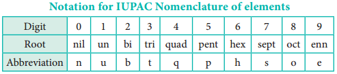
2. The numerical roots corresponding to the atomic number are put together and ‘ium’ is added as suffix

3. The final ‘n’ of ‘enn’ is omitted when it is written before ‘nil’ (enn + nil = enil) similarly the final ‘i’ of ‘bi’ and ‘tri’ is omitted when it written before ‘ium’ (bi + ium = bium; tri + ium = trium)

4. The symbol of the new element is derived from the first letter of the numerical roots.

The following table illustrates these facts.

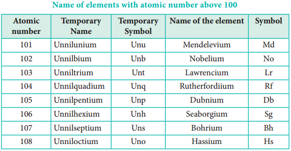
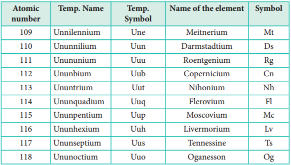
To overcome all these difficulties, IUPAC nomenclature has been recommended for all the elements with Z > 100. It was decided by IUPAC that the names of elements beyond atomic number 100 should use Latin words for their numbers. The names of these elements are derived from their numerical roots.

Fermium is a synthetic element with the symbol Fm and atomic number 100. It is an actinide and the heaviest element that can be formed by neutron bombardment of lighter elements, and hence the last element that can be prepared in macroscopic quantities, although pure fermium metal has not yet been prepared.

The twelve elements of nature are Earth, Water, Wind, Fire, Thunder, Ice, Force, Time, Flower, Shadow, Light and Moon.

Uranium

The heaviest element known to occur in nature is uranium, which contains only 92 protons, putting it 30 places below the putative new element in the periodic table. In the laboratory, physicists have managed to create elements up to 118, but they are all highly unstable.

The fifth element on top of earth, air, fire, and water, is space or aether. It was hard for people to believe that the stars and everything else in space were made of the other elements, so space was considered as a fifth element.

According to ancient and medieval science, aether also spelled ether, aither, or ether and also called quintessence (fifth element), is the material that fills the region of the universe above the terrestrial sphere.

Find free online Chemistry Topics covering a broad range of concepts from research institutes around the world.

Moseley’s Work and Modern Periodic Law

In 1913, Henry Moseley studied the characteristic X-rays spectra of several elements by bombarding them with high energy electrons and observed a linear correlation between atomic number and the frequency of X-rays emitted which is given by the following expression.

\(\sqrt{υ}\) = a(Z – b)

Where, υ is the frequency of the X-rays emitted by the element with atomic number ‘Z’; a and b are constants and have same values for all the elements.

The plot of \(\sqrt{υ}\) against Z gives a straight line. Using this relationship, we can determine the atomic number of an unknown (new) element from the frequency of X-ray emitted. Based on his work, the modern periodic law was developed which states that, “the physical and chemical properties of the elements are periodic functions of their atomic numbers.” Based on this law, the elements were arranged in order of their increasing atomic numbers.

This mode of arrangement reveals an important truth that the elements with similar properties recur after regular intervals. The repetition of physical and chemical properties at regular intervals is called periodicity.

Modern Periodic Table

The physical and chemical properties of the elements are correlated to the arrangement of electrons in their outermost shell (valence shell). Different elements having similar outer shell electronic configuration possess similar properties. For example, elements having one electron in their valence shell s-orbital possess similar physical and chemical properties. These elements are grouped together in the modern periodic table as first group elements.

Similarly, all the elements are arranged in the modern periodic table which contains 18 vertical columns and 7 horizontal rows. The vertical columns are called groups and the horizontal rows are called periods. Groups are numbered 1 to 18 in accordance with the IUPAC recommendation which replaces the old numbering scheme IA to VIIA, IB to VIIB and VIII.

Each period starts with the element having general outer electronic configuration ns¹ and ends with ns² np⁶.
Here ‘n’ corresponds to the period number (principal quantum number). The aufbau principle and the  electronic configuration of atoms provide a theoretical foundation for the modern periodic table.

Find free online Chemistry Topics covering a broad range of concepts from research institutes around the world.

Classification of Elements

During the 19^th century, scientists have isolated several elements and the list of known elements increased. Currently, we have 118 known elements. Out of 118 elements, 92 elements with atomic numbers 1 to 92 are found in nature. Scientists have found out there are some similarities in properties among certain elements.

This observation has led to the idea of classification of elements based on their properties. In fact, classification will be beneficial for the effective utilization of these elements. Several attempts were made to classify the elements. However, classification based on the atomic weights led to the construction of a proper form of periodic table.

In 1817, J. W. Dobereiner classified some elements such as chlorine, bromine and iodine with similar chemical properties into the group of three elements called as triads. In triads, the atomic weight of the middle element nearly equal to the arithmetic mean of the atomic weights of the remaining two elements. However, only a limited number of elements can be grouped as triads.

This concept can not be extended to some triads which have nearly same atomic masses such as [Fe, Co, Ni], [Ru, Rh, Pd] and [Os, Ir, Pt].

In 1862, A. E. B. de Chancourtois reported a correlation between the properties of the elements and their atomic weights. He said ‘the properties of bodies are the properties of numbers’. He intended the term numbers to mean the value of atomic weights.

He designed a helix by tracing at an angle 45˚ to the vertical axis of a cylinder with circumference of 16 units. He arranged the elements in the increasing atomic weights along the helix on the surface of this cylinder.

One complete turn of a helix corresponds to an atomic weight increase of 16. Elements which lie on the 16 equidistant vertical lines drawn on the surface of cylinder shows similar properties. This was the first reasonable attempt towards the creation of periodic table. However, it did not attract much attention.

In 1864, J. Newland made an attempt to classify the elements and proposed the law of octaves. On arranging the elements in the increasing order of atomic weights, he observed that the properties of every eighth element are similar to the properties of the first element. This law holds good for lighter elements up to calcium.

Mendeleev’s Classification

In 1868, Lothar Meyer had developed a table of the elements that closely resembles the modern periodic table. He plotted the physical properties such as atomic volume, melting point and boiling point against atomic weight and observed a periodical pattern.

During same period Dmitri Mendeleev independently proposed that “the properties of the elements are the periodic functions of their atomic weights” and this is called periodic law. Mendeleev listed 70 elements, which were known till histime in several vertical columns in order of increasing atomic weights. Thus, Mendeleev constructed the first periodic table based on the periodic law.

As shown in the periodic table, he left some blank spaces since there were no known elements with the appropriate properties at that time. He and others predicted the physical and chemical properties of the missing elements. Eventually these missing elements were discovered and found to have the predicted properties.

For example, Gallium (Ga) of group III and germanium (Ge) of group IV were unknown at that time. But Mendeleev predicted their existence and properties. He referred the predicted elements as eka-aluminium and eka-silicon. After discovery of the actual elements, their properties were found to match closely to those predicted by Mendeleev (Table 3.4).

Properties predicted for Eka-aluminium and Eka-silicon

Anomalies of Mendeleev’s Periodic Table

Some elements with similar properties were placed in different groups and those with dissimilar properties were placed in same group. Similarly elements with higher atomic weights were placed before lower atomic weights based on their properties in contradiction to his periodic law. Example ⁵⁹Co₂₇ was placed before ^58.7Ni₂₈; Tellurium (127.6) was placed in VI group but Iodine (127.0) was placed in VII group.

Find free online Chemistry Topics covering a broad range of concepts from research institutes around the world.

Filling of Orbitals

In an atom, the electrons are filled in various orbitals according to aufbau principle, Pauli exclusion principle and Hund’s rule. These rules are described below.

Aufbau Principle:

The word Aufbau in German means ‘building up’. In the ground state of the atoms, the orbitals are filled in the order of their increasing energies. That is the electrons first occupy the lowest energy orbital available to them.

Once the lower energy orbitals are completely filled, then the electrons enter the next higher energy orbitals. The order of filling of various orbitals as per the Aufbau principle is given in the figure 2.12 which is in accordance with (n+ l) rule.

Pauli Exclusion Principle:

Pauli formulated the exclusion principle which states that “No two electrons in an atom can have the same set of values of all four quantum numbers.”

It means that, each electron must have unique values for the four quantum numbers (n, l, m and s). For the lone electron present in hydrogen atom, the four quantum numbers are: n = 1; l = 0; m = 0 and s = + ½. For the two electrons present in helium, one electron has the quantum numbers same as the electron of hydrogen atom, n = 1, l = 0, m = 0 and s = + ½. For other electron, the fourth quantum number is different i.e., n = 1, l = 0, m = 0 and s = – ½.

As we know that the spin quantum number can have only two values + ½ and – ½, only two electrons can be accommodated in a given orbital in accordance with Pauli exclusion principle. Let us understand this by writing all the four quantum numbers for the eight electron in L shell.

Hund’s Rule of Maximum Multiplicity

The Aufbau principle describes how the electrons are filled in various orbitals. But the rule does not deal with the filling of electrons in the degenerate orbitals (i.e. orbitals having same energy) such as p_x, p_y, p_z. In what order these orbitals to be filled? The answer is provided by the Hund’s rule of maximum multiplicity. It states that electron pairing in the degenerate orbitals does not take place until all the available orbitals contains
one electron each.

We know that there are three p orbitals, five d orbitals and seven f orbitals. According to this rule, pairing of electrons in these orbitals starts only when the 4^th, 6^th and 8^th electron enters the p, d and f orbitals respectively.

For example, consider the carbon atom which has six electrons. According to Aufbau principle, the electronic configuration is 1s², 2s², 2p² It can be represented as below,

In this case, in order to minimise the electron-electron repulsion, the sixth electron enters the unoccupied 2p_y orbital as per Hunds rule. i.e. it does not get paired with the fifth electron already present in the 2px orbital.

Electronic Configuration of Atoms

The distribution of electrons into various orbitals of an atom is called its electronic configuration. It can be written by applying the aufbau principle, Pauli exclusion principle and Hund’s rule. The electronic configuration is written as nl^x, where n represents the principle of quantum number, ‘l’ represents the letter designation of the orbital [s(l=0), p (l=1), d(l=2) and f(l=3)] and ‘x’ represents the number of electron present in that orbital.

Let us consider the hydrogen atom which has only one electron and it occupies the lowest energy orbital i.e. 1s according to aufbau principle. In this case n = 1; l = s; x = 1.

Hence the electronic configuration is 1s¹. (read as one-ess-one).

The orbital diagram for this configuration is,

The electronic configuration and orbital diagram for the elements upto atomic number 10 are given below:

The actual electronic configuration of some elements such as chromium and copper slightly differ from the expected electronic configuration in accordance with the Aufbau principle.

For chromium – 24

Expected Configuration:

1s² 2s² 2p⁶ 3s² 3p⁶ 3d⁴ 4s²

Actual Configuration:

1s² 2s² 2p⁶ 3s² 3p⁶ 3d⁵ 4s¹

For copper – 29

Expected Configuration:

1s² 2s² 2p⁶ 3s² 3p⁶ 3d⁹ 4s²

Actual Configuration:

1s² 2s² 2p⁶ 3s² 3p⁶ 3d¹⁰ 4s¹

The reason for above observed configuration is that fully filled orbitals and half filled orbitals have been found to have extra stability. In other words, p³, p⁶, d⁵, d¹⁰, f⁷ and f¹⁴ configurations are more stable than p², p⁵, d⁴, d⁹, f⁶ and f¹³. Due to this stability, one of the 4s electrons occupies the 3d orbital in chromium and copper to attain the half filled and the completely filled configurations respectively.

Stability of Half filled and Completely Filled Orbitals:

The exactly half filled and completely filled orbitals have greater stability than other partially filled configurations in degenerate orbitals. This can be explained on the basis of symmetry and exchange energy. For example chromium has the electronic configuration of [Ar]3d⁵ 4s¹ and not [Ar]3d⁴ 4s² due to the symmetrical distribution and exchange energies of d electrons.

Symmetrical Distribution of Electron:

Symmetry leads to stability. The half filled and fully filled configurations have symmetrical distribution of electrons (Figure 2.13) and hence they are more stable than the unsymmetrical configurations.

The degenerate orbitals such as p_x, p_y, p_z have equal energies and their orientation in space are different
as shown in Figure 2.14. Due to this symmetrical distribution, the shielding of one electron on the other is relatively small and hence the electrons are attracted more strongly by the nucleus and it increases the stability.

Exchange Energy:

If two or more electrons with the same spin are present in degenerate orbitals, there is a possibility for exchanging their positions. During exchange process the energy is released and the released energy is called exchange energy. If more number of exchanges are possible, more exchange energy is released. More number of exchanges are possible only in case of half filled and fully filled configurations.

For example, in chromium the electronic confiuration is [Ar]3d⁵ 4s¹. The 3d orbital is half filled and there are ten possible exchanges as shown in Figure 2.15. On the other hand only six exchanges are possible for [Ar]3d⁴ 4s² configuration. Hence, exchange energy for the half filled confiuration is more. This increases the stability of half filled 3d orbitals.

The exchange energy is the basis for Hund’s rule, which allows maximum multiplicity, that is electron pairing is possible only when all the degenerate orbitals contain one electron each.

Find free online Chemistry Topics covering a broad range of concepts from research institutes around the world.

Quantum Numbers

The electron in an atom can be characterised by a set of four quantum numbers, namely principal quantum number (n), azimuthal quantum number (l), magnetic quantum number (m) and spin quantum number (s). When Schrodinger equation is solved for a wave function Ψ, the solution contains the first three quantum numbers n, l and m. The fourth quantum number arises due to the spinning of the electron about its own axis. However, classical pictures of species spinning around themselves are incorrect.

Principal Quantum Number (n):

This quantum number represents the energy level in which electron revolves around the nucleus and is denoted by the symbol ‘n’.

1. The ‘n’ can have the values 1, 2, 3, … n = 1 represents K shell; n = 2 represents L shell and n = 3, 4, 5 represent the M, N, O shells, respectively.

2. The maximum number of electrons that can be accommodated in a given shell is 2n².

3. ‘n’ gives the energy of the electron,

and the distance of the electron from the nucleus is given by

Azimuthal Quantum Number (l) or Subsidiary Quantum Number:

1. It is represented by the letter ‘l’, and can take integral values from zero to n-1, where n is the principal quantum number.
2. Each l value represents a subshell (orbital). l = 0, 1, 2, 3 and 4 represents the s, p, d, f and g orbitals respectively.
3. The maximum number of electrons that can be accommodated in a given subshell (orbital) is 2(2l + 1).
4. It is used to calculate the orbital angular momentum using the expression

Angular momentum = \(\sqrt{l(l+1)}\) \(\frac{h}{2π}\) …………. (2.4)

Magnetic Quantum Number (ml):

1. It is denoted by the letter ‘ml’. It takes integral values ranging from -l to +l through 0. i.e. if l = 1; m = -1, 0 and +1
2. Different values of m for a given l value, represent different orientation of orbitals in space.
3. The Zeeman Effect (the splitting of spectral lines in a magnetic field) provides the experimental justification for this quantum number.
4. The magnitude of the angular momentum is determined by the quantum number l while its direction is given by magnetic quantum number.

Spin Quantum Number (m_s):

1. The spin quantum number represents the spin of the electron and is denoted by the letter ‘m_s‘
2. The electron in an atom revolves not only around the nucleus but also spins. It is usual to write this as electron spins about its own axis either in a clockwise direction or in anti-clockwise direction.
3. The visualisation is not true. However spin is to be understood as representing a property that revealed itself in magnetic fields.
4. Corresponding to the clockwise and anti-clockwise spinning of the electron, maximum two values are possible for this quantum number.
5. The values of ‘m_s‘ is equal to -½ and + ½

Quantum Numbers and its Significance

Shapes of Atomic Orbitals:

The solution to Schrodinger equation gives the permitted energy values called eigen values and the wave functions corresponding to the eigen values are called atomic orbitals. The solution (Ψ) of the Schrodinger wave equation for one electron system like hydrogen can be represented in the following form in spherical polar coordinates r, θ, φ as,

Ψ (r, θ, φ) = R(r).f(θ).g(φ) ………….. (2.15)

(where R(r) is called radial wave function, other two functions are called angular wave functions)

As we know, the Ψ itself has no physical meaning and the square of the wave function |Ψ|² is related to the probability of finding the electrons within a given volume of space. Let us analyse how |Ψ|² varies with the distance from nucleus (radial distribution of the probability) and the direction from the nucleus (angular distribution of the probability).

Radial Distribution Function:

Consider a single electron of hydrogen atom in the ground state for which the quantum numbers are n = 1 and l = 0. i.e. it occupies 1s orbital. The plot of R(r)² versus r for 1s orbital is given in Figure 2.3

The graph shows that as the distance between the electron and the nucleus decreases, the probability of finding the electron increases. At r=0, the quantity R(r)² is maximum i.e. The maximum value for |Ψ|² is at the nucleus. However, probability of finding the electron in a given spherical shell around the nucleus is important. Let us consider the volume (dV) bounded by two spheres of radii r and r + dr.

Volume of the sphere, V = \(\frac{4}{3}\)πr³
\(\frac{dV}{dr}\) = \(\frac{4}{3}\)π(3r²)
dV = \(\frac{4}{3}\)π(3r²)
dV = 4πr²dr
Ψ²dV = 4πr²Ψ²dr ……………. (2.16)

The plot of 4πr². R(r)² versus r is given below.

The above plot shows that the maximum probability occurs at distance of 0.52 Å from the nucleus. This is equal to the Bohr radius. It indicates that the maximum probability of finding the electron around the nucleus is at this distance. However, there is a probability to find the electron at other distances also. The radial distribution function of 2s, 3s, 3p and 3d orbitals of the hydrogen atom are represented as follows.

For 2s orbital, as the distance from nucleus r increases, the probability density first increases, reaches a small maximum followed by a sharp decrease to zero and then increases to another maximum, after that decreases to zero.

The region where this probability density function reduces to zero is called nodal surface or a radial node. In general, it has been found that nsorbital has (n-1) nodes. In other words, number of radial nodes for 2s orbital is one, for 3s orbital it is two and so on. The plot of 4πr². R(r)² versus r for 3p and 3d orbitals shows similar pattern but the number of radial nodes are equal to(n-l-1) (where n is principal quantum number and l is azimuthal quantum number of the orbital).

Angular Distribution Function:

The variation of the probability of locating the electron on a sphere with nucleus at its centre depends on the azimuthal quantum number of the orbital in which the electron is present. For 1s orbital, l=0 and m=0. f(θ) = 1/\(\sqrt{2}\) and g(φ) = 1/\(\sqrt{2π}\).

Therefore, the angular distribution function is equal to 1/\(\sqrt{2π}\). i.e. it is independent of the angle θ and φ. Hence, the probability of finding the electron is independent of the direction from the nucleus. The shape of the s orbital is spherical as shown in the figure 2.7.

For p orbitals l = 1 and the corresponding m values are -1, 0 and +1. The angular distribution functions are quite complex and are not discussed here. The shape of the p orbital is shown in Figure 2.8. The three different m values indicates that there are three different orientations possible for p orbitals.

These orbitals are designated as p_x, p_y and p_z and the angular distribution for these orbitals shows that the lobes are along the x, y and z axis respectively. As seen in the Figure 2.8 the 2p orbitals have one nodal plane.

For ‘d’ orbital l = 2 and the corresponding m values are -2, -1, 0 +1,+2. The shape of the d orbital looks like a ‘clover leaf ‘. The five m values give rise to five d orbitals namely d_xy, d_yz, d_zx, d_x2-y2 and d_z2. The 3d orbitals contain two nodal planes as shown in Figure 2.9.

For ‘f ‘ orbital, l = 3 and the m values are -3, -2, -1, 0, +1, +2, +3 corresponding to seven f orbitals f_z³, f_xz²,
f_yz², f_xyz, f_z(x²-y²), f_x(x²-3y²), f_y(3x²-y²), which are shown in Figure 2.10. There are 3 nodal planes in the f-orbitals.

Energies of Orbitals

In hydrogen atom, only one electron is present. For such one electron system, the energy of the electron in the n^th orbit is given by the expression

From this equation, we know that the energy depends only on the value of principal quantum number. As the n value increases the energy of the orbital also increases. The energies of various orbitals will be in the following order:

1s < 2s = 2p < 3s = 3p = 3d < 4s = 4p = 4d = 4f < 5s = 5p = 5d = 5f < 6s = 6p = 6d = 6f < 7s

The electron in the hydrogen atom occupies the 1s orbital that has the lowest energy. This state is called ground state. When this electron gains some energy, it moves to the higher energy orbitals such as 2s, 2p etc… These states are called excited states.

However, the above order is not true for atoms other than hydrogen (multi-electron systems). For such systems the Schrodinger equation is quite complex. For these systems the relative order of energies of various orbitals is given approximately by the (n+l) rule.

It states that, the lower the value of (n + l) for an orbital, the lower is its energy. If two orbitals have the same value of (n + l), the orbital with lower value of n will have the lower energy. Using this rule the order of energies of various orbitals can be expressed as follows.

n+ l values of different orbitals

Based on the (n+ l) rule, the increasing order of energies of orbitals is as follows:

1s < 2s < 2p < 3s < 3p < 4s < 3d < 4p < 5s < 4d < 5p < 6s < 4f < 5d < 6p < 7s < 5f < 6d

As we know there are three different orientations in space that are possible for a p orbital. All the three p orbitals, namely, p_x, p_y and p_z have same energies and are called degenerate orbitals. However, in the presence of magnetic or electric field the degeneracy is lost.

In a multi-electron atom, in addition to the electrostatic attractive force between the electron and nucleus, there exists a repulsive force among the electrons. These two forces are operating in the opposite direction. This results in the decrease in the nuclear force of attraction on electron.

The net charge experienced by the electron is called effective nuclear charge. The effective nuclear charge depends on the shape of the orbitals and it decreases with increase in azimuthal quantum number l. The order of the effective nuclear charge felt by a electron in an orbital within the given shell is s > p > d > f. Greater the effective nuclear charge, greater is the stability of the orbital. Hence, within a given energy level, the energy of the orbitals are in the following order. s < p < d < f.

The energies of same orbital decrease with an increase in the atomic number. For example, the energy of the 2s orbital of hydrogen atom is greater than that of 2s orbital of lithium and that of lithium is greater than that of sodium and so on, that is, E_2s(H) > E_2s(Li) > E_2s(K).

Find free online Chemistry Topics covering a broad range of concepts from research institutes around the world.

Quantum Mechanical Model of Atom – Schrodinger Equation:

The motion of objects that we come across in our daily life can be well described using classical mechanics which is based on the Newton’s laws of motion. In classical mechanics the physical state of the particle is defined by its position and momentum. If we know both these properties, we can predict the future state of the system based on the force acting on it using classical mechanics.

However, according to Heisenberg’s uncertainty principle both these properties cannot be measured simultaneously with absolute accuracy for a microscopic particle such as an electron. The classical mechanics does not consider the dual nature of the matter which is significant for microscopic particles.

As a consequence, it fails to explain the motion of microscopic particles. Based on the Heisenberg’s principle and the dual nature of the microscopic particles, a new mechanics called quantum mechanics was developed.

Erwin Schrodinger expressed the wave nature of electron in terms of a differential equation. This equation determines the change of wave function in space depending on the field of force in which the electron moves. The time independent Schrödinger equation can be expressed as,

\(\hat {H} \)Ψ = EΨ ………….. (2.12)

Where \(\hat {H} \) is called Hamiltonian operator, Ψ is the wave function and is a funciton of position Ψ(x, y, z) E is the energy of the system

The above schrodinger wave equation does not contain time as a variable and is referred to as time independent Schrodinger wave equation. This equation can be solved only for certain values of E, the total energy. i.e. the energy of the system is quantised. The permitted total energy values are called eigen values and corresponding wave functions represent the atomic orbitals.

Main Features of the Quantum Mechanical Model of Atom

1. The energy of electrons in atoms is quantised

2. The existence of quantized electronic energy levels is a direct result of the wave like properties of electrons. The solutions of Schrodinger wave equation gives the allowed energy levels (orbits).

3. According to Heisenberg uncertainty principle, the exact position and momentum of an electron can not be determined with absolute accuracy. As a consequence, quantum mechanics introduced the concept of orbital. Orbital is a three dimensional space in which the probability of finding the electron is maximum.

4. The solution of Schrodinger wave equation for the allowed energies of an atom gives the wave function ψ, which represents an atomic orbital. The wave nature of electron present in an orbital can be well defined by the wave function ψ.

5. The wave function ψ itself has no physical meaning. However, the probability of finding the electron in a small volume dxdydz around a point (x, y, z) is proportional to |ψ(x, y, z)|² dxdydz around a point (x, y, z) is proportional to |ψ(x, y, z)|² is known as probability density and is always positive.

Find free online Chemistry Topics covering a broad range of concepts from research institutes around the world.

Heisenberg’s Uncertainty Principle

The dual nature of matter imposes a limitation on the simultaneous determination of position and momentum of a microscopic particle. Based on this, Heisenberg arrived at his uncertainty principle, which states that ‘It is impossible to accurately determine both the position and the momentum of a microscopic particle simultaneously’. The product of uncertainty (error) in the measurement is expressed as follows.

Δx.Δp ≥ h/4π …………….. (2.11)

where, Δx and Δp are uncertainties in determining the position and momentum, respectively.

The uncertainty principle has negligible effect for macroscopic objects and becomes significant only for microscopic particles such as electrons. Let us understand this by calculating the uncertainty in the velocity of the electron in hydrogen atom. (Bohr radius of 1^st orbit is 0.529 Ǻ) Assuming that the position of the electron in this orbit is determined with the accuracy of 0.5 % of the radius.

Uncertainity in Position = ∆x
= \(\frac{0.5%}{100%}\) × 0.529 Ǻ
= \(\frac{0.5}{100}\) × 0.529 × 10^-10m
Δx = 2.645 × 10^-13m

From the Heisenberg’s uncertainity principle,
Δx.Δp ≥ \(\frac{h}{4π}\)
Δx.(m.Δv) ≥ \(\frac{h}{4π}\)

Δv ≥ 2.189 × 10⁸ ms^-1

Therefore, the uncertainty in the velocity of the electron is comparable with the velocity of light. At this high level of uncertainty it is very difficult to find out the exact velocity.

Find free online Chemistry Topics covering a broad range of concepts from research institutes around the world.

Wave Particle Duality of Matter

Albert Einstein proposed that light has dual nature. i.e. light photons behave both like a particle and as a wave. Louis de Broglie extended this concept and proposed that all forms of matter showed dual character. To quantify this relation, he derived an equation for the wavelength of a matter wave. He combined the following two equations of energy of which one represents wave character (hυ) and the other represents the particle nature (mc²).

(i) Planck’s quantum hypothesis:
E = hυ ……………. (2.6)

(ii) Einstein’s mass-energy relationship
E = mc² …………….. (2.7)

From (2.6) and (2.7)

hν = mc²
hc/λ = mc²
λ = h/mc …………….. (2.8)

The equation 2.8 represents the wavelength of photons whose momentum is given by mc (Photons have zero rest mass)

For a particle of matter with mass m and moving with a velocity v, the equation 2.8 can be written as
λ = h/mv ………………. (2.9)

This is valid only when the particle travels at speeds much less than the speed of Light.

This equation implies that a moving particle can be considered as a wave and a wave can exhibit the properties (i.e momentum) of a particle. For a particle with high linear momentum (mv) the wavelength will be so small and cannot be observed. For a microscopic particle such as an electron, the mass is of the order of 10^-31 kg, hence the wavelength is much larger than the size of atom and it becomes significant.

Let us understand this by calculating de Broglie wavelength in the following two cases:

• A 6.626 kg iron ball moving at 10 ms^-1
• An electron moving at 72.73 ms^-1

λ_ironball= h/mv

λ_electron= h/mv

For the electron, the de Broglie wavelength is significant and measurable while for the iron ball it is too small to measure, hence it becomes insignificant.

According to the de Broglie concept, the electron that revolves around the nucleus exhibits both particle and wave character. In order for the electron wave to exist in phase, the circumference of the orbit should be an integral multiple of the wavelength of the electron wave. Otherwise, the electron wave is out of phase.

Circumference of the orbit = nλ

2πr = nλ ……………… (2.10)
2πr = nh/mv

Rearranging,
mvr = nh/2π …………… (2.11)

Angular momentum = nh/2π

The above equation was already predicted by Bohr. Hence, De Broglie and Bohr’s concepts are in agreement with each other.

Davison and Germer Experiment:

The wave nature of electron was experimentally confirmed by Davisson and Germer. They allowed the accelerated beam of electrons to fall on a nickel crystal and recorded the diffraction pattern. The resultant diffraction pattern is similar to the x-ray diffraction pattern. The finding of wave nature of electron leads to the development of various experimental techniques such as electron microscope, low energy electron diffraction etc.

Find free online Chemistry Topics covering a broad range of concepts from research institutes around the world.

Introduction to Atom Models

Let us recall the history of the development of atomic models from the previous classes. We know that all things are made of matter. The basic unit that makes up all matter is atom. The word ‘atom’ has been derived from the Greek word ‘a – tomio’ meaning nondivisible.

Atom was considered as nondivisible until the discovery of subatomic particles such as electron, proton and neutron. J. J. Thomson’s cathode ray experiment revealed that atoms consist of negatively charged particles called electrons.

He proposed that atom is a positively charged sphere in which these electrons are embedded like the seeds in the watermelon. Later, Rutherford’s α-ray scattering experiment results proved that Thomson’s model was wrong. Rutherford bombarded a thin gold foil with a stream of fast moving α-particles. It was observed that

1. Most of the α-particles passed through the foil
2. Some of them were deflected through a small angle and
3. Very few α-particles were reflected back by 180°

Based on these observations, he proposed that in an atom there is a tiny positively charged nucleus and the electrons are moving around the nucleus with high speed. The theory of electromagnetic radiation states that a moving charged particle should continuously loose its energy in the form of radiation.

Therefore, the moving electron in an atom should continuously loose its energy and finally collide with nucleus resulting in the collapse of the atom. However, this doesn’t happen and the atoms are stable. Moreover, this model does not explain the distribution of electrons around the nucleus and their energies.

Bohr Atom Model:

The work of Planck and Einstein showed that the energy of electromagnetic radiation is quantised in units of hν (where ν is the frequency of radiation and h is Planck’s constant 6.626 × 10^-34 Js). Extending Planck’s quantum hypothesis to the energies of atoms, Niels Bohr proposed a new atomic model for the hydrogen atom. This model is based on the following assumptions:

1. The energies of electrons in an atom are quantised.

2. The electron is revolving around the nucleus in a certain circular path of fixed energy called stationary orbit.

3. Electron can revolve only in those orbits in which the angular momentum (mvr) of the electron must be equal to an integral multiple of h/2π.

i.e. mvr = nh/2π ……………… (2.1)
where n = 1, 2, 3, … etc.,

4. As long as an electron revolves in the fixed stationary orbit, it doesn’t lose its energy. However, when an electron jumps from higher energy state (E₂) to a lower energy state (E₁), the excess energy is emitted as radiation. The frequency of the emitted radiation is

E₂ – E₁ = hυ
and
υ = \(\frac{(E₂)-E₁)}{h}\) ………………. (2.2)

Conversely, when suitable energy is supplied to an electron, it will jump from lower energy orbit to a higher energy orbit.

Applying Bohr’s postulates to a hydrogen like atom (one electron species such as H, He⁺ and Li²⁺ etc..) the radius of the n^th orbit and the energy of the electron revolving in the n^th orbit were derived.

The results are as follows:

The detailed derivation of r_n and E_n will be discussed in 12^th standard atomic physics unit.

Limitation of Bohr’s Atom Model:

The Bohr’s atom model is applicable only to species having one electron such as hydrogen, Li²⁺ etc… and not applicable to multi electron atoms. It was unable to explain the splitting of spectral lines in the presence of magnetic field (Zeeman effect) or an electric field (Stark effect).

Bohr’s theory was unable to explain why the electron is restricted to revolve around the nucleus in a fixed orbit in which the angular momentum of the electron is equal to nh/2π and a logical answer for this, was provided by Louis de Broglie.

Find free online Chemistry Topics covering a broad range of concepts from research institutes around the world.

Oxidation Number Defination and Examples

It is defined as the imaginary charge left on the atom when all other atoms of the compound have been removed in their usual oxidation states that are assigned according to set of rules. A term that is often used interchangeably with oxidation number is oxidation state.

1. The oxidation state of a free element (i.e. in its uncombined state) is zero.
Example: each atom in H₂, Cl₂, Na, S₈ have the oxidation number of zero.

2. For a monatomic ion, the oxidation state is equal to the net charge on the ion.

Example:

The oxidation number of sodium in Na⁺ is +1.

The oxidation number of chlorine in Cl^– is -1.

3. The algebric sum of oxidation states of all atoms in a molecule is equal to zero, while in ions, it is equal to the net charge on the ion.

Example:

In H₂SO₄; 2 × (oxidation number of hydrogen) + (oxidation number of S) + 4 (oxidation number of oxygen) = 0.

In SO₄^2-; (oxidation number of S) + 4 (oxidation number of oxygen) = – 2.

4. Hydrogen has an oxidation number of +1 in all its compounds except in metal hydrides where it has – 1 value.

Example:

Oxidation number of hydrogen in hydrogen chloride (HCl) is + 1.
Oxidation number of hydrogen in sodium hydride (NaH) is -1.

5. Fluorine has an oxidation state of – 1 in all its compounds.

6. The oxidation state of oxygen in most compounds is – 2. Exceptions are peroxides, super oxides and compounds with fluorine.

Example:

Oxidation number of oxygen,

(i) in water (H₂O) is – 2.

(ii) in hydrogen peroxide (H₂O₂) is -1.
2 (+ 1) + 2x = 0;
⇒ 2x = – 2;
⇒ x = – 1

(iii) in super oxides such as KO₂ is – 1
+1 + 2x = 0;
2x = – 1;
x = – 1/2

(iv) in oxygen difloride (OF₂) is + 2.
x + 2 (- 1) = 0;
x = + 2

7. Alkali metals have an oxidation state of + 1 and alkaline earth metals have an oxidation state of + 2 in all their compounds.

Calculation of Oxidation Number Using the Above Rules.

Redox Reactions in Terms of Oxidation Numbers

During redox reactions, the oxidation number of elements changes. A reaction in which oxidation number of the element increases is called oxidation. A reaction in which it decreases is called reduction.

Consider the following reaction

In this reaction, manganese in potassium permanganate (KMnO₄) favours the oxidation of ferrous sulphate (FeSO₄) into ferric sulphate (Fe₂(SO₄)₃ by gaining electrons and thereby gets reduced. Such reagents are called oxidising agents or oxidants. Similarly, the reagents which facilitate reduction by releasing electrons and get oxidised are called reducing agents.

Types of Redox Reactions

Redox reactions are classified into the following types.

1. Combination Reactions:

Redox reactions in which two substances combine to form a single compound are called combination reaction.

Example:

2. Decomposition Reactions:

Redox reactions in which a compound breaks down into two or more components are called decomposition reactions. These reactions are opposite to combination reactions. In these reactions, the oxidation number of the different elements in the same substance is changed.

Example

3. Displacement Reactions:

Redox reactions in which an ion (or an atom) in a compound is replaced by an ion (or atom) of another element are called displacement reactions. They are further classified into

• Metal Displacement Reactions
• Non-Metal Displacement Reactions

Metal Displacement Reactions:

Place a zinc metal strip in an aqueous copper sulphate solution taken in a beaker. Observe the solution, the intensity of blue colour of the solution slowly reduced and finally disappeared. The zinc metal strip became coated with brownish metallic copper. This is due to the following metal displacement reaction.

Non-Metal Displacement

4. Disproportionation Reaction (Auto Redox Reactions)

In some redox reactions, the same compound can undergo both oxidation and reduction. In such reactions, the oxidation state of one and the same element is both increased and decreased. These reactions are called disproportionation reactions.

Examples

5. Competitive Electron Transfer Reaction

In metal displacement reactions, we learnt that zinc replaces copper from copper sulphate solution. Let us examine whether the reverse reaction takes place or not. As discussed earlier, place a metallic copper strip in zinc sulphate solution. If copper replaces zinc from zinc sulphate solution, Cu²⁺ ions would be released into the solution and the colour of the solution would change to blue.

But no such change is observed. Therefore, we conclude that among zinc and copper, zinc has more tendency to release electrons and copper to accept the electrons.

Let us extend the reaction to copper metal and silver nitrate solution. Place strip of metallic copper in sliver nitrate solution taken in a beaker. After some time, the solution slowly turns blue. This is due to the formation of Cu²⁺ ions, i.e. copper replaces silver from silver nitrate.

The reaction is,

It indicates that between copper and silver, copper has the tendency to release electrons and silver to accept electrons.

From the above experimental observations, we can conclude that among the three metals, namely, zinc, copper and silver, the electron releasing tendency is in the following order.

Zinc > Copper > Silver

This kind of competition for electrons among various metals helps us to design (galvanic) cells. In XII standard we will study the galvanic cell in detail.

Balancing (the Equation) of Redox Reactions

The two methods for balancing the equation of redox reactions are as follows.

• The oxidation number method
• Ion-electron method / half reaction method.

Both are based on the same principle:

In oxidation – reduction reactions the total number of electrons donated by the reducing agent is equal to the total number of electrons gained by
the oxidising agent.

Oxidation Number Method

In this method, the number of electrons lost or gained in the reaction is calculated from the oxidation numbers of elements before and after the reaction. Let us consider the oxidation of ferrous sulphate by potassium permanganate in acid medium. The unbalanced chemical equation is,

FeSO₄ + KMnO₄ + H₂SO₄ → Fe₂(SO₄)₃ + MnSO₄ + K₂SO₄ + H₂O

Step 1

Using oxidation number concept, identify the reactants (atom) which undergo oxidation and reduction.

(a) The oxidation number of Mn in KMnO₄ changes from +7 to +2 by gaining five electrons.

(b) The oxidation number of Fe in FeSO₄ changes from +2 to +3 by loosing one electron.

Step 2

Since, the total number of electrons lost is equal to the total number of electrons gained, equate, the number of electrons, by cross multiplication of the respective formula with suitable integers on reactant side as below. Here, the product Fe₂(SO₄)₃ contains 2 moles of iron, So, the Coefficients 1e^– & 5e^– are multiplied by the number ‘2’.

10 FeSO₄ + 2 KMnO₄ + H₂SO₄ → Fe₂(SO₄)₃ + MnSO₄ + K₂SO₄ + H₂O

Step 3

Balance the reactant / Product Oxidised / Reduced

Now, based on the reactant side, balance the products (ie oxidised and reduced).The above equation becomes

10FeSO₄ + 2KMnO₄ + H₂SO₄ → 5Fe₂(SO₄)₃ + 2MnSO₄ + K₂SO₄ + H₂O

Step 4

Balance the other elements except H and O atoms. In this case, we have to balance K and S atoms but K is balanced automatically.

Reactant Side:

10 ‘S’ atoms (10 FeSO₄)

Product Side:

18 ‘S’ atoms

5Fe₂(SO₄)₃ + 2MnSO₄ + K₂SO₄

15S + 2S + 1S = 18S

Therefore the difference 8-S atoms in reactant side, has to be balanced by multiplying H₂SO₄ by ‘8’ The equation now becomes,

10FeSO₄ + 2KMnO₄ + 8H₂SO₄ → 5Fe₂(SO₄)₃ + 2MnSO₄ + K₂SO₄ + H₂O

Step 5

Balancing ‘H’ and ‘O’ atoms

Reactant side ’16’-H atoms (8H₂SO₄ i.e. 8 × 2H = 16 ‘H’)

Product side ‘2’ – H atoms (H₂O i.e. 1 × 2H = 2 ‘H’)

Therefore, multiply H₂O molecules in the product side by ‘8’

10 FeSO₄ + 2 KMnO₄ + 8 H₂SO₄ → 5 Fe₂(SO₄)₃ + 2 MnSO₄ + k₂SO₄ + 8H₂O

The oxygen atom is automatically balanced. This is the balanced equation.

Ion – Electron Method

This method is used for ionic redox reactions.

Step 1

Using oxidation number concept, find out the reactants which undergo oxidation and reduction.

Step 2

Write two separate half equations for oxidation and reduction reaction, Let us consider the same example which we have already discussed in
oxidation number method.

KMnO₄ + FeSO₄ + H₂SO₄ → MnSO₄ + Fe₂(SO₄)₃ + K₂SO₄ + H₂O

The ionic form of this reaction is,

The two half reactions are,

Fe²⁺ → Fe³⁺ + 1e^– ………………….. (1)
and
MnO^–₄ + 5e^– → Mn²⁺ …………………. (2)

Balance the atoms and charges on both sides of the half reactions.

Equation (1) ⇒ No changes i.e.,

Fe²⁺ → Fe³⁺ + 1e^– ………………….. (1)

Equation (2) ⇒ 4’O’ on the reactant side, therefore add 4H₂O on the product side, to balance ‘H’ – add, 8H⁺ in the reactant side

MnO^–₄ + 5e^– + 8H⁺ → Mn²⁺ + 4H₂O ……………… (3)

Step 3

Equate both half reactions such that the number of electrons lost is equal to number of electrons gained. Addition of two half reactions gives the balanced equation represented by equation (6).

Find free online Chemistry Topics covering a broad range of concepts from research institutes around the world.

Redox Reaction Examples, Types and Applications

When an apple is cut, it turns brown after sometime. Do you know the reason behind this colour change? It is because of a chemical reaction called oxidation. We come across oxidation reactions in our daily life. For example

1. Burning of LPG gas
2. Rusting of iron
3. Oxidation of carbohydrates, lipids, etc. into CO₂ and H₂O to produce energy in the living organisms.

All oxidation reactions are accompanied by reduction reactions and vice versa. Such reactions are called redox reactions. As per the classical concept, addition of oxygen (or) removal of hydrogen is called oxidation and the reverse is called reduction.

Fig. 1.4 Oxidation reactions in daily life

Consider the following two reactions.

Reaction 1:
4 Fe + 3O₂ → 2 Fe₂O₃

Reaction 2:
H₂S + Cl₂ → 2 HCl + S

Both these reactions are oxidation reactions as per the classical concept. In the first reaction which is responsible for the rusting of iron, the oxygen adds on to the metal, iron. In the second reaction, hydrogen is removed from Hydrogen sulphide (H₂S). Identity which species gets reduced.

Consider the following two reactions in which the removal of oxygen and addition of hydrogen take place respectively. These reactions are called reduction reactions as per the classical concept.

CuO + C → Cu + CO (Removal of oxygen from cupric oxide)

S + H₂ → H2S (Addition of hydrogen to sulphur)

Oxidation-reduction reactions i.e. redox reactions are not always associated with oxygen or hydrogen. In such cases, the process can be explained on the basis of electrons. The reaction involving loss of electron is termed oxidation and gain of electron is termed reduction.

For example,

Fe²⁺ → Fe³⁺ + e^– (loss of electron-oxidation).
Cu²⁺ + 2e^– → Cu (gain of electron-reduction)

Redox reactions can be better explained using oxidation numbers.